idplot
Syntax
Description
Plot Data
idplot( plots the input and output
channels of the data data)data. data can be a
timetable, a comma-separated matrix pair, a single matrix, or an iddata object.
The function plots the outputs on the top axes and the inputs on the bottom axes. When
data is a timetable, the software assumes that the last variable is
the sole output channel and that the remaining variables are the input channels. If you
have data that does not fit this pattern, specify the channels using the
InputName and OutputName name-value arguments.
For time-domain data, the input and output signals are plotted as a function of time. The specification for the input intersample behavior (
InputInterSampleoption indataPlotOptionswhendatais a timetable or numeric matrix pair,data.InterSamplewhendatais aniddata object) determines whether the input signals are plotted as linearly interpolated curves or as staircase plots. For example, ifdata.InterSample = 'zoh', the input is piecewise constant between sampling points, and is plotted accordingly.For frequency-domain data, the magnitude and phase of each input and output signal are plotted over the available frequency span.
To plot a subset of the data, use subreferencing:
idplot(data(201:300,:))plots all the variables in the samples 201 to 300 in the timetable objectdata.idplot(udata(201:300,:),ydata(201:300,:))plots the samples 201 to 300 in the matrix pairdata.idplot(data(201:300))plots the samples 201 to 300 in theiddataobjectdata.idplot(data(201:300,'Altitude',{'Angle_of_attack','Speed'}))plots the specified samples of the output namedAltitudeand the inputs namedAngle_of_attackandSpeed.idplot(data(:,[3 4],[3:7]))plots all samples of output channel numbers 3 and 4 and input numbers 3 through 7.
idplot(data1,...,dataN) plots multiple datasets. The number of
plot axes is determined by the number of unique input and output names among all the
datasets.
idplot(data1,LineSpec1...,dataN,LineSpecN) specifies the line
style, marker type, and color for each dataset. You can specify options for only some data
sets. For example, idplot(data1,data2,'k',data3) specifies black as the
plot color for data2.
Use Plot Handle to Specify Axes
idplot( plots
into the axes with the handle axes_handle,___)axes_handle instead of into the current
axes (gca). Use this syntax with any of the input argument
combinations in the previous syntaxes.
Specify Additional Model Options
sys = idplot(___,Name,Value)
For example, specify output and input channels using the name-value arguments
OutputName and InputName. Use this syntax when
data is a timetable and does not follow the default software
interpretation of the last variable being the sole output channel and all other channels
being input channels.
If you specify 'OutputName' and all the other variables in
data are input channels, you do not need to specify
'InputName'.
Specify Plot Options
idplot(___,
specifies the plot options.plotoptions)
Return Plot Handle
h = idplot(___)getoptions and
setoptions.
Examples
Load the data in tt1, which is a timetable.
load sdata1 tt1;
Plot the data.
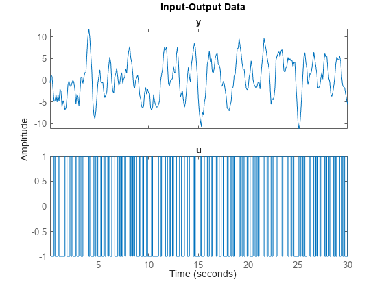
idplot(tt1)
The function plots the output on the top axes and the input on the bottom axes.
Plot the first 100 samples.
idplot(tt1(1:100,:))
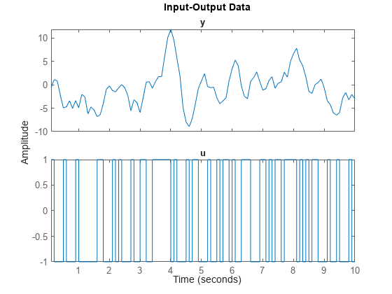
Only the first 100 samples appear in the plot.
You can undock and right-click the plot to explore characteristics such as peak and mean values.
Load the data in umat1 and ymat1, which are numeric input and output matrices, and the sample time in Ts.
load sdata1 umat1 ymat1 Ts
Plot only the input.
idplot(umat1,[],'Ts',Ts)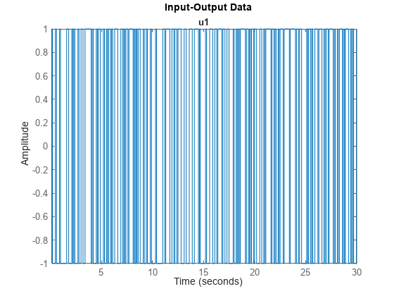
Plot only the output.
idplot([],ymat1,'Ts',Ts)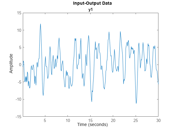
Plot the input and output together.
idplot(umat1,ymat1,'Ts',Ts)
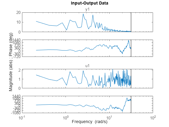
Load the data.
load iddata1 z1
Convert the data to the frequency domain.
zf = fft(z1);
Plot the data.
idplot(zf);
Timetable Data
Load two data sets.
load sdata1 tt1
load sdata2 tt2
Plot both datasets.
idplot(tt1,tt2)
Because the data sets use the same input and output names, the function plots both data sets together.
Specify unique input and output names.
tt1.Properties.VariableNames = {'tt1_input' 'tt1_output'};
tt2.Properties.VariableNames = {'tt2_input' 'tt2_output'};
Plot both datasets.
idplot(tt1,tt2)
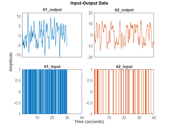
The function plots the data sets separately.
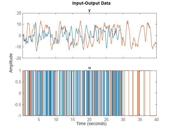
Matrix Data
Load two data sets.
load sdata1 umat1 ymat1
load sdata2 umat2 ymat2
Plot both datasets.
idplot(umat1,ymat1,umat2,ymat2)

The function plots both data sets together. Because Ts is not included in the previous command, the software assumes that the sample time is 1 second.
iddata Data
Load two data sets.
load iddata1 z1
load iddata2 z2
Plot both datasets.
plot(z1,z2)
Because the data sets use the same input and output names, the function plots both data sets together.
Specify unique input and output names.
z1.InputName = "z1_input";
z2.InputName = "z2_input";
z1.OutputName = "z1_output";
z2.OutputName = "z2_output";
Plot both datasets.
plot(z1,z2)


The function plots the data sets separately.
Create a multiexperiment data set.
load iddata1 z1
load iddata2 z2
zm = merge(z1,z2);
Plot the data.
idplot(zm)
legend('show')
For multiexperiment data, each experiment is treated as a separate data set. You can right-click the plots to view their characteristics.
Load the timetable ttsteam, which contains two input variables and two output variables. View the variable names.
load steamdata ttsteam
ttsteam.Properties.VariableNames
ans = 1×4 cell
    {'Pressure'}    {'MagVolt'}    {'GenVolt'}    {'Speed'}
The output variables are GenVolt and Speed. The input variables are Pressure and Magvolt.
Try plotting the variables without specifying input and output names.
idplot(ttsteam)
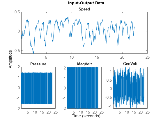
The software assumes that only the last variable, 'Speed', is an output. Use the 'InputName' and 'OutputName' name-value arguments to specify the corresponding variables.
InputName = {"Pressure" "MagVolt"};
OutputName = {"GenVolt" "Speed"};
idplot(ttsteam,'InputName',InputName,'OutputName',OutputName)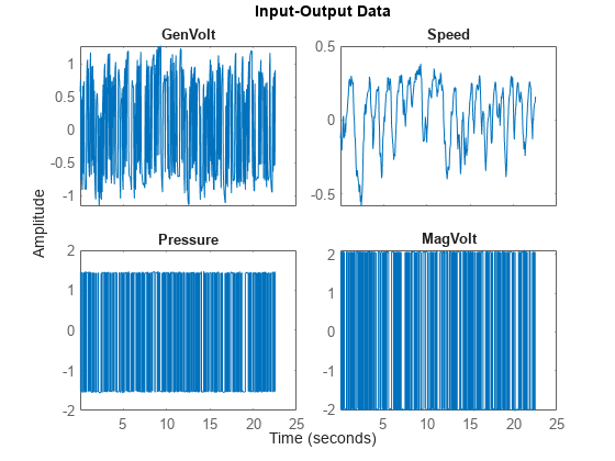
In this case, since all the variables in ttsteam are either inputs or outputs, you can also specify only the outputs. The software interprets the remaining variables as inputs.
idplot(ttsteam,'OutputName',OutputName)
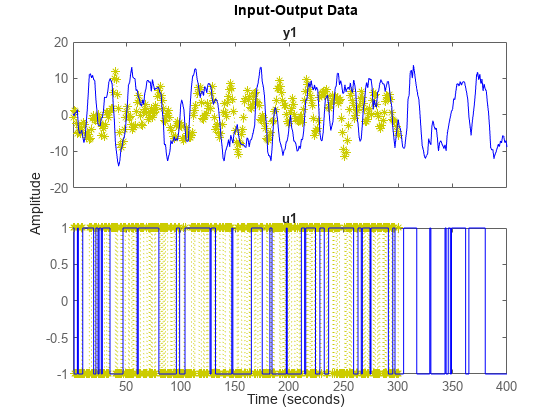
Load two data sets.
load sdata1 umat1 ymat1;
load sdata2 umat2 ymat2;
Specify the line style for both data sets.
idplot(umat1,ymat1,'y:*',umat2,ymat2,'b')
Create a figure with two subplots and return the handles for each subplot axes in s.
figure % new figure
s(1) = subplot(1,2,1); % left subplot
s(2) = subplot(1,2,2); % right subplot
Load the data sets.
load sdata1 tt1;
load sdata2 tt2;
Create a data plot in each axes using the handles.
idplot(s(1),tt1)
idplot(s(2),tt2)
Configure a time plot.
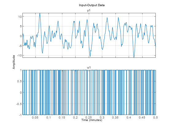
opt = dataPlotOptions('time');Specify minutes as the time unit of the plot.
opt.TimeUnits = 'minutes';Turn the grid on.
opt.Grid = 'on';Create the plot with the options specified by opt.
load sdata1 umat1 ymat1 Ts
idplot(umat1,ymat1,'Ts',Ts,opt);
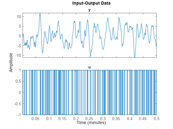
Create a data plot and return the handle.
load sdata1 tt1;
h = idplot(tt1);

Set the time unit of the plot.
setoptions(h,'TimeUnits','minutes');
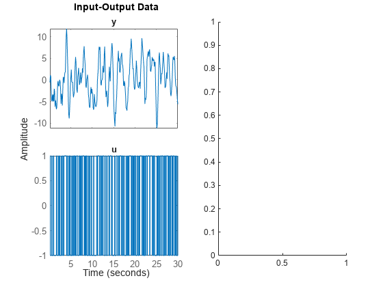
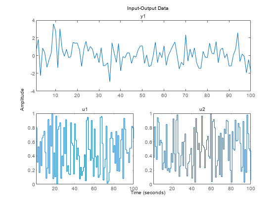
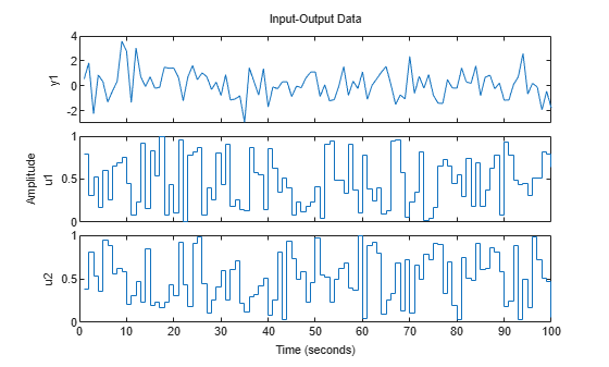
Generate data with two inputs and one output.
z = iddata(randn(100,1),rand(100,2));
Configure a time plot.
opt = iddataPlotOptions('time');Plot the data.
h = idplot(z,opt);
Change the orientation of the plots such that all inputs are plotted in one column, and all outputs are in a second column.
opt.Orientation = 'two-column';
h = idplot(z,opt);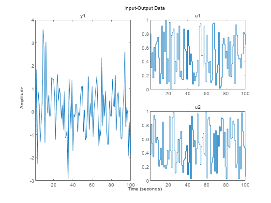
Alternatively, use setoptions.
setoptions(h,'Orientation','two-column')
You can also change the orientation by right-clicking the plot and choosing Orientation in the context menu.
Input Arguments
Name-Value Arguments
Output Arguments
Tips
Right-clicking the plot opens the context menu, where you can access the following options and plot controls.
| Option | Description and Suboptions |
|---|---|
| Datasets | View the datasets used in the plot. |
| Characteristics | Peak Value — View the peak value of the data. This value is useful for transient data. Mean Value — View the mean value of the data. This value is useful for steady-state data. |
| Orientation | For data with one input and one output channel:
For data with more than one input or output channel:
|
| I/O Grouping | Group input and output channels on the plot. Use this option with datasets with more than one input or output channel. |
| I/O Selector | Select a subset of the input and output channels to plot. By default, all input and output channels are plotted. Use this option with data sets with more than one input or output channel. |
| Grid | Add grids to your plot. |
| Normalize | Normalize the y-scale of all data in the plot. |
| Properties | Open the Property Editor dialog box, where you can customize plot attributes. |