Main Content

spectrumest

Estimate transfer function model for power spectrum data

Since R2022b

Description

Estimate Model

sys = spectrumest(data) fits a minimum-phase, discrete-time transfer function model, sys, to the power spectrum data in data. The spectrumest function assumes that data is measured uniformly over a frequency range of 0 to π rad/s. spectrumest determines the order (number of poles) of sys automatically.

sys = spectrumest(data,w) specifies the frequency vector w of the data.

sys = spectrumest(data,w,ts) specifies the sample time ts of the data.

  • To estimate discrete-time transfer functions, set ts > 0.

  • To estimate continuous-time transfer functions, set ts = 0.

example

sys = spectrumest(data,w,ts,np) fits a transfer function with np poles to the data. spectrumest also fits np zeros to the data.

sys = spectrumest(data,w,ts,np,nz) fits a transfer function with np poles and nz zeros to the data.

Enable Feedthrough

sys = spectrumest(data,w,ts,Feedthrough=ft) specifies whether the identified transfer function sys has feedthrough. To enable feedthrough, sys must be discrete time (ts > 0).

sys = spectrumest(data,w,ts,np,nz,Feedthrough=ft) specifies whether the transfer function with np poles and nz zeros has feedthrough.

Specify Additional Options

example

sys = spectrumest(___,options) specifies estimation configuration options, such as the numerical search method to be used for estimation. Specify opt after all other arguments shown in previous syntaxes.

Examples

collapse all

Fit transfer functions models of varying orders to power spectrum data, and compare the resulting spectral models.

Load the benchmark Marple data. Extract the power spectrum from the data, along with the corresponding frequency points and sample time.

load marple
fsys = etfe(marple);
ps = squeeze(fsys.SpectrumData);
w = fsys.Frequency;
Ts = fsys.Ts;

Fit a fourth-order spectral model to the data.

sys1 = spectrumest(ps,w,Ts,4);

Fit a second, more detailed spectral model to the data. Use a spectrumestOptions object to apply an inverse weighting filter to the estimated model. Do not specify a number of poles.

opt = spectrumestOptions(WeightingFilter='inv');
sys2 = spectrumest(ps,w,Ts,opt);

spectrumest generates a plot of model orders (number of poles) to use to estimate the model. The optimal model order identified by spectrumest is selected.

  1. Under Chosen Order, optionally select a different model order.

  2. Click Apply.

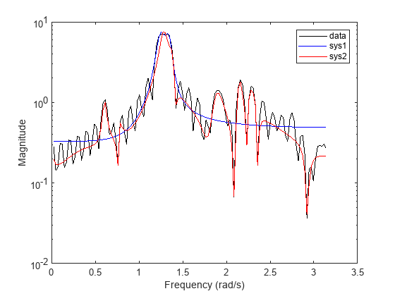
Plot the data and the frequency responses of the two spectral models on a semilog plot. The higher-order model produces a more accurate fit to the power spectrum data.

semilogy(w,sqrt(ps),'k', ...
    w,squeeze(abs(freqresp(sys1,w))),'b', ...
    w,squeeze(abs(freqresp(sys2,w))),'r')
xlabel('Frequency (rad/s)')
ylabel('Magnitude')
legend('data','sys1','sys2')

Figure contains an axes object. The axes object contains 3 objects of type line. These objects represent data, sys1, sys2.

Input Arguments

collapse all

Power spectrum data, specified as a nonnegative real vector.

Frequency points corresponding to data, specified as a numeric vector in units of rad/TimeUnit, where TimeUnit is the system time unit that was used to compute data.

spectrumest assumes the Nyquist frequency to be equal to w(end).

Sample time of data, in seconds, specified as a nonnegative real scalar.

  • If data is a continuous-time spectrum, specify ts = 0. The output transfer function sys has the form

    H(s) = num(s) / den(s),

    where num and den are the numerator and denominator polynomial coefficients in descending powers of s.

  • If data is a discrete-time spectrum, specify ts > 0 so that π/ts represents the Nyquist frequency. The output transfer function has the form

    H(z-1) = num(z-1)/den(z-1),

    where num and den are the numerator and denominator polynomial coefficients in descending powers of z-1.

The default value of ts depends on whether you specify the spectrum frequencies w:

  • If you specify w, then ts = π / w(end).

  • If you do not specify w, then ts = 1.

Number of poles to fit to the transfer function sys to determine its model order, specified as one of these values:

  • "best" — Pick the number of poles required to set an optimal order automatically. The number of poles is in the range 1:length(H)/2.

  • Nonnegative integer — Apply a fixed order to sys by fitting the specified number of poles to it.

  • Vector of nonnegative integers — Generate a bar plot to pick the optimal order based on the significant singular values of a Loewner matrix generated for the data.

If you specify np without nz, then spectrumest fits np zeros to sys.

Example: [1:10]

Number of zeros to fit to the transfer function sys, specified as a nonnegative integer.

  • If data is a discrete-time spectrum (ts > 0), then nz represents the number of zeros of the numerator polynomial expressed in the z–1 variable. For example, P(z–1) = 1 + 2z–1 + 3z–2 has 2 zeros.

  • If np is a scalar value and nz is not specified, then nz = np.

  • If np is set to "best" or a range of values, then the nz argument is ignored and instead determined as follows:

    • If ts = 0 and ft is false, then nz = np – 1.

    • In all other cases, nz = np.

Option to enable feedthrough in transfer function sys, specified as logical 1 (true) or logical 0 (false).

This argument applies only for discrete-time systems (ts > 0). For continuous-time systems (ts = 0), the presence of feedthrough is implied by np = nz.

Estimation options, specified as a spectrumestOptions option set. Options that you specify include:

  • Display of estimation progress

  • Weighting prefilter

  • Numerical search method to be used in estimation

Output Arguments

collapse all

Identified spectral model transfer function, returned as an idtf object.

Version History

Introduced in R2022b