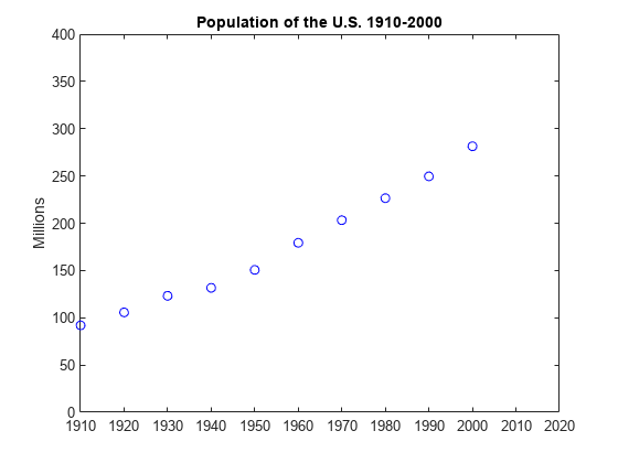
Predicting the US Population
This example shows that extrapolating data using polynomials of even modest degree is risky and unreliable.
This example is older than MATLAB®. It started as an exercise in Computer Methods for Mathematical Computations, by Forsythe, Malcolm and Moler, published by Prentice-Hall in 1977.
Now, MATLAB makes it much easier to vary the parameters and see the results, but the underlying mathematical principles are unchanged.
Create and plot two vectors with US Census data from 1910 to 2000.
% Time interval
t = (1910:10:2000)';

% Population
p = [91.972 105.711 123.203 131.669 150.697...
    179.323 203.212 226.505 249.633 281.422]';

% Plot
plot(t,p,'bo');
axis([1910 2020 0 400]);
title('Population of the US 1910-2000');
ylabel('Millions');

What is your guess for the population in the year 2010?
p
p = 10×1

   91.9720
  105.7110
  123.2030
  131.6690
  150.6970
  179.3230
  203.2120
  226.5050
  249.6330
  281.4220
Fit the data with a polynomial in t and use it to extrapolate the population at t = 2010. Obtain the coefficients in the polynomial by solving a linear system of equations involving an 11-by-11 Vandermonde matrix, with elements as powers of scaled time, A(i,j) = s(i)^(n-j).
n = length(t);
s = (t-1950)/50;
A = zeros(n);
A(:,end) = 1;
for j = n-1:-1:1
   A(:,j) = s .* A(:,j+1);
end
Obtain the coefficients c for a polynomial of degree d that fits the data p by solving a linear system of equations involving the last d+1 columns of the Vandermonde matrix:
A(:,n-d:n)*c ~= p
If
d < 10, then more equations than unknowns exist, and a least-squares solution is appropriate.If
d == 10, then you can solve the equations exactly and the polynomial actually interpolates the data.
In either case, use the backslash operator to solve the system. The coefficients for the cubic fit are:
c = A(:,n-3:n)\p
c = 4×1

   -5.7042
   27.9064
  103.1528
  155.1017
Now evaluate the polynomial at every year from 1910 to 2010 and plot the results.
v = (1910:2020)';
x = (v-1950)/50;
w = (2010-1950)/50;
y = polyval(c,x);
z = polyval(c,w);

hold on
plot(v,y,'k-');
plot(2010,z,'ks');
text(2010,z+15,num2str(z));
hold off

Compare the cubic fit with the quartic. Notice that the extrapolated point is very different.
c = A(:,n-4:n)\p;
y = polyval(c,x);
z = polyval(c,w);

hold on
plot(v,y,'k-');
plot(2010,z,'ks');
text(2010,z-15,num2str(z));
hold off

As the degree increases, the extrapolation becomes even more erratic.
cla
plot(t,p,'bo')
hold on
axis([1910 2020 0 400])
colors = hsv(8);
labels = {'data'};
for d = 1:8
   [Q,R] = qr(A(:,n-d:n));
   R = R(1:d+1,:);
   Q = Q(:,1:d+1);
   c = R\(Q'*p);    % Same as c = A(:,n-d:n)\p;
   y = polyval(c,x);
   z = polyval(c,11);
   plot(v,y,'color',colors(d,:));
   labels{end+1} = ['degree = ' int2str(d)];
end
legend(labels, 'Location', 'NorthWest')
hold off
