Main Content

etree

Elimination tree

Description

p = etree(A) returns an elimination tree of the square symmetric matrix whose upper triangle is that of A.

example

p = etree(A,type) specifies the type of elimination tree. For example, if type is "lo", then etree uses the lower triangle of A to construct the square symmetric matrix.

example

[p,q] = etree(___) also returns the postorder permutation q of the elimination tree. You can specify two outputs with any of the input argument combinations in the previous syntaxes.

Examples

collapse all

Create a 7-by-7 tridiagonal matrix of zeros and ones.

A = diag(ones(1,7)) + diag(ones(1,6),1) + diag(ones(1,6),-1)
A = 7×7

     1     1     0     0     0     0     0
     1     1     1     0     0     0     0
     0     1     1     1     0     0     0
     0     0     1     1     1     0     0
     0     0     0     1     1     1     0
     0     0     0     0     1     1     1
     0     0     0     0     0     1     1

Calculate an elimination tree of A. Each element p(i) of the elimination tree represents the parent of node i. p(7) is 0 because node 7 is the root of the tree.

p = etree(A)
p = 1×7

     2     3     4     5     6     7     0

Create a 6-by-6 block diagonal matrix of zeros and ones.

a = ones(3);
b = zeros(3);
B = [a b; b a]
B = 6×6

     1     1     1     0     0     0
     1     1     1     0     0     0
     1     1     1     0     0     0
     0     0     0     1     1     1
     0     0     0     1     1     1
     0     0     0     1     1     1

Calculate an elimination tree of B. etree returns a forest with two elimination trees, indicated by the root nodes at indices 3 and 6.

r = etree(B)
r = 1×6

     2     3     0     5     6     0

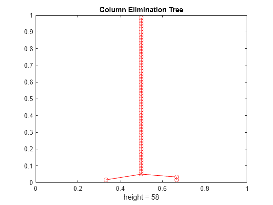
Calculate two different elimination trees of the bucky sparse matrix. The "lo" elimination tree uses the lower triangle of A, while the "col" elimination tree uses the matrix A'*A.

A = bucky;
p1 = etree(A,"lo");
p2 = etree(A,"col");

Plot the elimination trees using treeplot.

treeplot(p1)
title("Lower Triangle Elimination Tree")

Figure contains an axes object. The axes object with title Lower Triangle Elimination Tree, xlabel height = 58 contains 2 objects of type line. One or more of the lines displays its values using only markers

treeplot(p2)
title("Column Elimination Tree")

Figure contains an axes object. The axes object with title Column Elimination Tree, xlabel height = 58 contains 2 objects of type line. One or more of the lines displays its values using only markers

Calculate elimination trees of two permutations of the bucky sparse matrix. Use symrcm to create the symmetric reverse Cuthill-McKee ordering, and use symamd to create the symmetric approximate minimum degree ordering.

A = bucky;
r = symrcm(A);
p1 = etree(A(r,r));
m = symamd(A);
p2 = etree(A(m,m));

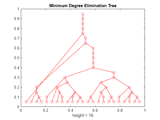
Plot the elimination trees using treeplot. The reverse Cuthill-McKee elimination tree is a line of nodes, while the minimum degree elimination tree has multiple disjoint branches.

treeplot(p1)
title("Reverse Cuthill-McKee Elimination Tree")

Figure contains an axes object. The axes object with title Reverse Cuthill-McKee Elimination Tree, xlabel height = 59 contains 2 objects of type line. One or more of the lines displays its values using only markers

treeplot(p2)
title("Minimum Degree Elimination Tree")

Figure contains an axes object. The axes object with title Minimum Degree Elimination Tree, xlabel height = 18 contains 2 objects of type line. One or more of the lines displays its values using only markers

Plot the sparsity patterns using spy. The elimination tree of a matrix depends on its sparsity pattern, so the different sparsity patterns result in different elimination trees.

spy(A(r,r))
title("Reverse Cuthill-McKee Sparsity Pattern")

Figure contains an axes object. The axes object with title Reverse Cuthill-McKee Sparsity Pattern, xlabel nz = 180 contains a line object which displays its values using only markers.

spy(A(m,m))
title("Minimum Degree Sparsity Pattern")

Figure contains an axes object. The axes object with title Minimum Degree Sparsity Pattern, xlabel nz = 180 contains a line object which displays its values using only markers.

Input Arguments

collapse all

Input matrix. A can be either full or sparse. If the elimination tree type is "sym" or "lo", then A must be a square matrix. etree uses the sparsity structure of A to calculate the elimination tree.

Data Types: double | logical
Complex Number Support: Yes

Type of elimination tree, specified as "sym", "lo", "col", or "row". Use this argument to specify what matrix etree uses to compute the elimination tree.

  • If type is "sym", then etree constructs a square symmetric matrix using the upper triangle of A and returns the elimination tree of that matrix.

  • If type is "lo", then etree constructs a square symmetric matrix using the lower triangle of A and returns the elimination tree of that matrix.

  • If type is "col", then etree constructs the matrix A'*A and returns the elimination tree of that matrix, which is the column elimination tree of A.

  • If type is "row", then etree constructs the matrix A*A' and returns the elimination tree of that matrix, which is the row elimination tree of A.

Output Arguments

collapse all

Elimination tree, returned as a numeric vector. p(i) represents the parent of node i in the tree, or 0 if i is a root.

Postorder permutation of elimination tree p, returned as a numeric vector.

You can use the postorder permutation of an elimination tree when computing the columns of a Cholesky factorization by hand. For a node i and its parent node j in an elimination tree p, column i must be completely computed before column j in the Cholesky factorization. The postorder permutation of p specifies an order in which to compute these columns that is consistent with this requirement. Use chol to compute the factorization directly.

More About

collapse all

Elimination Tree

An elimination tree is a data structure that captures row and column dependencies of a Cholesky factorization and describes the operations that can be performed at the same time. Disjoint branches of an elimination tree can be calculated in parallel, so factorizations of matrices that have elimination trees with branching can be computed faster. You can reorder a sparse matrix to change the amount of fill-in and compute a different elimination tree.

References

[1] Chen, Yanqing, Timothy A. Davis, William W. Hager, and Sivasankaran Rajamanickam. “Algorithm 887: CHOLMOD, Supernodal Sparse Cholesky Factorization and Update/Downdate.” ACM Transactions on Mathematical Software 35, no. 3 (October 2008): 1–14. https://doi.org/10.1145/1391989.1391995.

[2] Pothen, Alex, and Sivan Toledo. "Elimination Structures in Scientific Computing." In Handbook of Data Structures and Applications, edited by Dinesh P. Mehta and Sartaj Sahni, 945–965. New York: Chapman and Hall/CRC, 2017. https://doi.org/10.1201/9781315119335

Extended Capabilities

Version History

Introduced before R2006a

Go to top of page