faceNormal
Triangulation unit normal vectors
Description
F = faceNormal( returns the unit
normal vectors to all triangles in a 2-D triangulation. The
TR)faceNormal function supports 2-D triangulations only.
F is a three-column matrix where each row contains the unit
normal coordinates corresponding to a triangle in
TR.ConnectivityList.
Examples
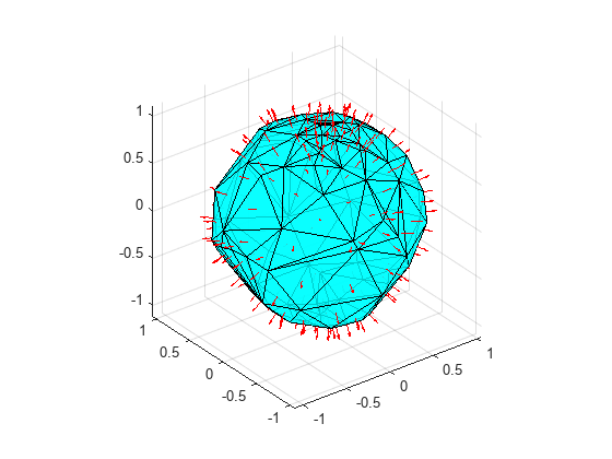
Compute and plot the unit normal vectors to the facets of a triangulation on a spherical surface.
Create a set of points on a spherical surface.
rng default;
theta = rand([100,1])*2*pi;
phi = rand([100,1])*pi;
x = cos(theta).*sin(phi);
y = sin(theta).*sin(phi);
z = cos(phi);
Triangulate the sphere using the delaunayTriangulation function.
DT = delaunayTriangulation(x,y,z);
Find the free boundary facets of the triangulation, and use them to create a 2-D triangulation on the surface.
[T,Xb] = freeBoundary(DT);
TR = triangulation(T,Xb);
Compute the centers and face normals of each triangular facet in TR.
P = incenter(TR);
F = faceNormal(TR);
Plot the triangulation along with the centers and face normals.
trisurf(T,Xb(:,1),Xb(:,2),Xb(:,3), ...
        FaceColor="cyan",FaceAlpha=0.8);
axis equal
hold on
quiver3(P(:,1),P(:,2),P(:,3), ...
        F(:,1),F(:,2),F(:,3), ...
        0.5,Color="r");
Input Arguments
Extended Capabilities
Version History
Introduced in R2013a