MPC Control of Aircraft with Unstable Poles
This example shows how to use an MPC controller to control an unstable aircraft with saturating actuators.
For an example that controls the same plant using an explicit MPC controller, see Explicit MPC Control of Aircraft with Unstable Poles.
Define Aircraft Model
The following linear time-invariant model is derived from the linearization of the longitudinal dynamics of an aircraft at an altitude of 3000 ft and a velocity of 0.6 Mach, [1]. The open-loop model has the following state-space matrices:
A = [-0.0151 -60.5651 0 -32.174;
     -0.0001 -1.3411 0.9929 0;
      0.00018 43.2541 -0.86939 0;
      0      0       1      0];
B = [-2.516 -13.136;
     -0.1689 -0.2514;
     -17.251 -1.5766;
      0        0];
C = [0 1 0 0;
     0 0 0 1];
D = [0 0;
     0 0];
The inputs, states, and outputs of the linear model represent deviations from their respective nominal values at the nonlinear model operating point.
Here, the state variables are:
forward velocity (ft/sec)
attack angle (deg)
pitch rate (deg/sec)
pitch angle (deg)
The manipulated variables are the elevator and flaperon angles, in degrees. The attack and pitch angles are measured outputs to be regulated.
Create the plant, and specify the initial states as zero.
plant = ss(A,B,C,D);
x0 = zeros(4,1);
The open-loop system is unstable.
damp(plant)
         Pole              Damping       Frequency      Time Constant
                                       (rad/seconds)      (seconds)

 -7.50e-03 + 5.56e-02i     1.34e-01       5.61e-02         1.33e+02
 -7.50e-03 - 5.56e-02i     1.34e-01       5.61e-02         1.33e+02
  5.45e+00                -1.00e+00       5.45e+00        -1.83e-01
 -7.66e+00                 1.00e+00       7.66e+00         1.30e-01
Specify Controller Constraints
Both manipulated variables are constrained between +/- 25 degrees. Use scale factors to facilitate MPC tuning. Typical choices of scale factors are the upper/lower limit of the operating range.
MV = struct('Min',{-25,-25},'Max',{25,25},'ScaleFactor',{50,50});
Specify the scale factors for the plant outputs.
OV = struct('ScaleFactor',{60,60});
Specify Controller Tuning Weights
The control task is to get zero offset for piecewise-constant references, while avoiding instability due to input saturation. Because both MV and OV variables are already scaled in the MPC controller, MPC weights are dimensionless and applied to the scaled MV and OV values. For this example, emphasize tracking of the attack angle by specifying a larger weight than the one used for the pitch angle.
Weights = struct('MV',[0 0],'MVRate',[0.1 0.1],'OV',[200 10]);
Create MPC Controller
Create an MPC controller with the specified plant model, a sample time of 0.05 sec. (20 Hz), a prediction horizon of 10 steps, a control horizon of 2 steps, and the previously specified weights, constraints and scale factors.
mpcobj = mpc(plant,0.05,10,2,Weights,MV,OV);
Calculate Closed Loop DC Gain Matrix
Calculate the steady state output sensitivity of the closed loop. A zero value means that the measured plant output can track the desired output reference setpoint.
cloffset(mpcobj)
-->Converting model to discrete time.
-->Integrator added as output disturbance model for measured output #1.
-->Integrator added as output disturbance model for measured output #2.
-->"Model.Noise" is empty. Assuming white noise on each measured output.

ans =

   1.0e-11 *

    0.0147    0.0028
    0.1956   -0.0084
Simulate Using Simulink
Use Simulink® to simulate the closed-loop response to a step of 0.1 and 2 degrees on the reference signals for the attack and pitch angles, respectively.
Open the Simulink model and set the MPC Controller property to mpcobj. For this example, the property is already set.
mdl = 'mpc_aircraft';
open_system(mdl)
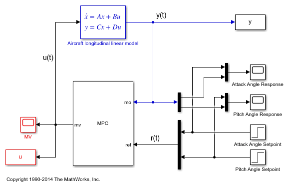
Simulate the system from the command line using the Simulink sim command.
sim(mdl)
Open the scopes showing the manipulated variables and the aircraft output response.
open_system('mpc_aircraft/MV')
open_system('mpc_aircraft/Attack Angle Response')
open_system('mpc_aircraft/Pitch Angle Response')
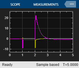
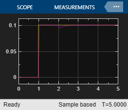

As expected, the closed-loop response shows good setpoint tracking performance for both channels.
References
[1] P. Kapasouris, M. Athans, and G. Stein, "Design of feedback control systems for unstable plants with saturating actuators", Proc. IFAC Symp. on Nonlinear Control System Design, Pergamon Press, pp.302--307, 1990
[2] A. Bemporad, A. Casavola, and E. Mosca, "Nonlinear control of constrained linear systems via predictive reference management", IEEE® Trans. Automatic Control, vol. AC-42, no. 3, pp. 340-349, 1997.
bdclose(mdl)