Heat Transfer in Orthotropic Material Plate due to Laser Beam

Open Live Script

Find the temperature distribution on a square plate made of orthotropic material. A laser beam hits the middle of the plate and generates a heat flux. This example shows how to

Specify an orthotropic thermal conductivity that also depends on the temperature using a conductivity matrix and a function handle.
Define a heat flux pulse of a Gaussian shape using a function handle. The example shows a function modeling a beam with the steady amplitude that is switched off after a particular time, as well as a function modeling the beam with its amplitude gradually decaying over time.

Thermal Analysis Setup

Create and plot a geometry representing a 40-by-40-by-3 cm plate.

L = 0.4; % m
W = 0.4; % m
H = 0.03; % m
g = multicuboid(L,W,H);
figure
pdegplot(g,FaceLabels="on",FaceAlpha=0.3)

Create a finite element analysis model with the plate geometry for transient thermal analysis.

model = femodel(AnalysisType="thermalTransient",Geometry=g);

Specify the initial temperature of the plate, 300 K.

model.CellIC = cellIC(Temperature=300);

Generate a mesh.

model = generateMesh(model);

Specify the heat flux boundary condition on top of the plate. First, specify a heat flux as a short pulse created by the laser beam by using the heatFluxSteady function. See Heat Flux Functions.

model.FaceLoad(2) = faceLoad(Heat = @heatFluxSteady);

Plot the heat flux returned by heatFluxSteady at the initial time t = 0 s.

a = linspace(-L/2,L/2);
b = linspace(-W/2,W/2);
[x,y] = meshgrid(a,b);
location.x = x;
location.y = y;
state.time = 0;
flux = heatFluxSteady(location,state);
figure
contourf(x,y,flux,100,LineStyle="none")
colorbar
xlabel("x")
ylabel("y")

Isotropic Thermal Conductivity

First, assume that the plate is made of an isotropic material with the thermal conductivity 50 $W / (m \cdot K)$ .

K = 50;

Specify the material properties. The mass density of the plate is 1960 $k g / m^{3}$ , and the specific heat is 710 $J / (k g \cdot K)$ .

model.MaterialProperties = ...
    materialProperties(ThermalConductivity=K, ...
                       MassDensity=1960, ...
                       SpecificHeat=710);

Solve the thermal problem for the times between 0 and 2 seconds.

t = 0:0.1:2;
Rt_iso = solve(model,t);

Plot the results using the Visualize PDE Results Live Editor task. First, create a new live script by clicking the New Live Script button in the File section on the Home tab.

On the Live Editor tab, select Task > Visualize PDE Results. This action inserts the task into your script.

To plot the temperature of the plate:

In the Select results section of the task, select Rt_iso from the drop-down list.
In the Specify data parameters section of the task, set Type to Temperature.
Select the Animate checkbox to see how the temperature changes over time.

Orthotropic Thermal Conductivity

For orthotropic thermal conductivity, create a vector of thermal conductivity components $k_{x}$ , $k_{y}$ , and $k_{z}$ .

kx = 50; % W/(m*K)
ky = 50; % W/(m*K)
kz = 500; % W/(m*K)
K = [kx;ky;kz];

Specify material properties of the plate.

model.MaterialProperties = ...
    materialProperties(ThermalConductivity=K, ... % W/(m*K)
                       MassDensity=1960, ...      % kg/(m^3)
                       SpecificHeat=710);         % J/(kg*K)

Solve the thermal problem.

Rt_ortho = solve(model,t);

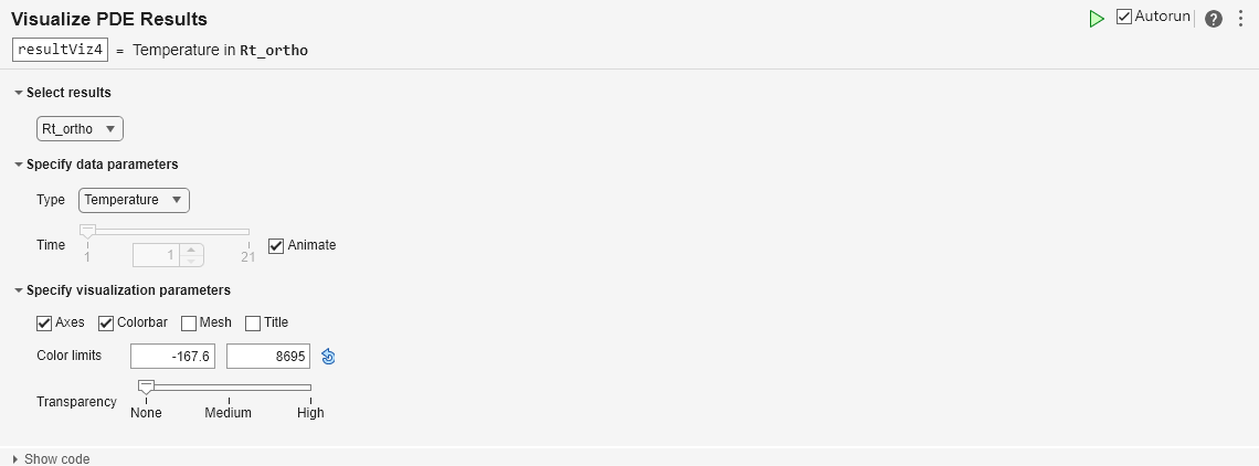
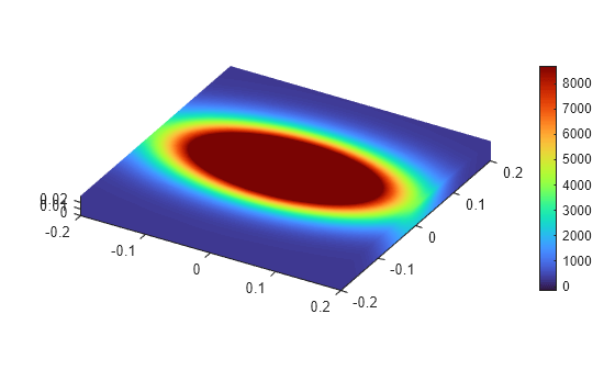
Plot the results using the Visualize PDE Results Live Editor task.

In the Select results section of the task, select Rt_ortho from the drop-down list.
In the Specify data parameters section of the task, set Type to Temperature.
Select the Animate checkbox to see how the temperature changes over time.

Orthotropic Thermal Conductivity Depending on Temperature

For orthotropic thermal conductivity that also depends on temperature, create a vector of thermal conductivity components $k_{x}$ , $k_{y}$ , and $k_{z}$ and use it in a function handle to account for temperature dependency.

kx = 50; % W/(m*K)
ky = 50; % W/(m*K)
kz = 500; % W/(m*K)
K = @(location,state) [kx;ky;kz] - 0.005*state.u;

Specify material properties of the plate.

model.MaterialProperties = ...
    materialProperties(ThermalConductivity=K, ... % W/(m*K)
                       MassDensity=1960, ...      % kg/(m^3)
                       SpecificHeat=710);         % J/(kg*K)

Solve the thermal problem.

Rt_ortho_t = solve(model,t);

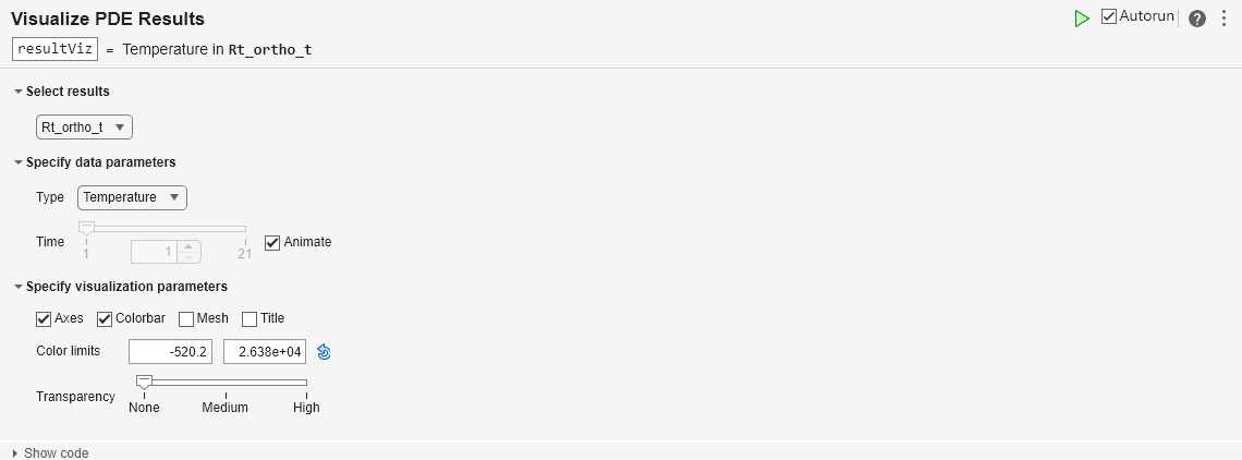
Plot the results using the Visualize PDE Results Live Editor task.

In the Select results section of the task, select Rt_ortho_t from the drop-down list.
In the Specify data parameters section of the task, set Type to Temperature.
Select the Animate checkbox to see how the temperature changes over time.

Thermal Pulse with Amplitude Decay

Now specify a heat flux as a pulse with the amplitude gradually decaying over time by using the heatFluxTimeDependent function. See Heat Flux Functions.

model.FaceLoad(2) = faceLoad(Heat = @heatFluxTimeDependent);

Visualize the heat flux for all time steps by creating an animation. Keep a fixed vertical scale by scaling all plots to use the maximum amplitude 350000000 $W / m^{2}$ as a colorbar upper limit.

state.time = t;
flux = heatFluxTimeDependent(location,state);
figure
for index = 1:length(t)
    contourf(x,y,flux(:,:,index),100,LineStyle="none")
    colorbar
    clim([0 350000000])
    xlabel("x")
    ylabel("y")
    M(index) = getframe;
end

To play the animation, use the movie(M) command.

Solve the thermal problem.

Rt = solve(model,t);

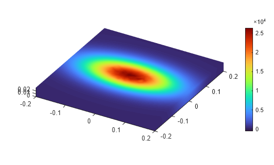
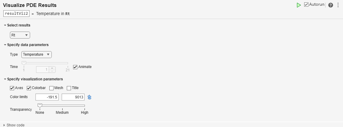
Plot the results using the Visualize PDE Results Live Editor task.

In the Select results section of the task, select Rt from the drop-down list.
In the Specify data parameters section of the task, set Type to Temperature.
Select the Animate checkbox to see how the temperature changes over time.

Heat Flux Functions

Create a function representing a Gaussian heat flux with the center at (x0,y0) and the maximum amplitude 350000000 $W / m^{2}$ . The heat flux has a steady amplitude for 0.03 seconds, then it switches off.

function fluxValSteady = heatFluxSteady(location,state)
A = 350000000;
x0 = 0;
y0 = 0;
sx = 0.1; % standard deviation along x
sy = 0.05; % standard deviation along y

fluxValSteady = A*exp(-(((location.x-x0).^2/(2*sx^2))+ ...
                        ((location.y-y0).^2/(2*sy^2))));

% Beam switches off after 0.03 seconds
    if state.time > 0.03   
        fluxVal = 0*location.x;
    end
end

Create a function representing a Gaussian heat flux with the center at (x0,y0) and with the amplitude 350000000 $W / m^{2}$ amplitude gradually decaying over time.

function fluxValTime = heatFluxTimeDependent(location,state)
t = state.time;
A = 350000000;
x0 = 0;
y0 = 0;
sx = 0.1; % standard deviation along x
sy = 0.05; % standard deviation along y
    for index = 1:length(t)
        fluxValTime(:,:,index) = A*exp(-(((location.x-x0).^2/(2*sx^2)) + ...
                                         ((location.y-y0).^2/(2*sy^2)))).*exp(-t(index));
    end
end