phased.MVDRBeamformer

Narrowband minimum-variance distortionless-response beamformer

Description

The phased.MVDRBeamformer System object™ implements a narrowband minimum-variance distortionless-response (MVDR) beamformer. The MVDR beamformer is also called the Capon beamformer. An MVDR beamformer belongs to the family of constrained optimization beamformers.

To beamform signals arriving at an array:

1. Create the phased.MVDRBeamformer object and set its properties.

2. Call the object with arguments, as if it were a function.

To learn more about how System objects work, see What Are System Objects?

Creation

Syntax

beamformer = phased.MVDRBeamformer

beamformer = phased.MVDRBeamformer(Name,Value)

Description

beamformer = phased.MVDRBeamformer creates an MVDR beamformer System object, beamformer, with default property values.

beamformer = phased.MVDRBeamformer(Name,Value) creates an MVDR beamformer with each property Name set to a specified Value. You can specify additional name-value pair arguments in any order as (Name1,Value1,...,NameN,ValueN). Enclose each property name in single quotes.

Example: beamformer = phased.MVDRBeamformer('SensorArray',phased.URA,'OperatingFrequency',300e6) sets the sensor array to a uniform rectangular array (URA) with default URA property values. The beamformer has an operating frequency of 300 MHz.

Properties

Unless otherwise indicated, properties are nontunable, which means you cannot change their values after calling the object. Objects lock when you call them, and the release function unlocks them.

If a property is tunable, you can change its value at any time.

For more information on changing property values, see System Design in MATLAB Using System Objects.

SensorArray — Sensor array

phased.ULA array with default property values (default) | Phased Array System Toolbox™ array

Sensor array, specified as an array System object belonging to Phased Array System Toolbox. The sensor array can contain subarrays.

Example: phased.URA

PropagationSpeed — Signal propagation speed (meters/second)

physconst('LightSpeed') (default) | real-valued positive scalar

Signal propagation speed, specified as a real-valued positive scalar. Units are in meters per second. The default propagation speed is the value returned by physconst('LightSpeed').

Example: 3e8

Data Types: single | double

OperatingFrequency — Operating frequency (Hz)

300e6 (default) | positive scalar

Operating frequency, specified as a positive scalar. Units are in Hz.

Example: 1e9

Data Types: single | double

DiagonalLoadingFactor — Diagonal loading factor

0 (default) | nonnegative scalar

Diagonal loading factor, specified as a nonnegative scalar. Diagonal loading is a technique used to achieve robust beamforming performance, especially when the sample size is small. A small sample size can lead to an inaccurate estimate of the covariance matrix. Diagonal loading also provides robustness due to steering vector errors. The diagonal loading technique adds a positive scalar multiple of the identity matrix to the sample covariance matrix.

Tunable: Yes

Data Types: single | double

TrainingInputPort — Enable training data input

false (default) | true

Enable training data input, specified as false or true. When you set this property to true, use the training data input argument, XT, when running the object. Set this property to false to use the input data, X, as the training data.

Data Types: logical

DirectionSource — Source of beamforming direction

'Property' (default) | 'Input port'

Source of beamforming direction, specified as 'Property' or 'Input port'. Specify whether the beamforming direction comes from the Direction property of this object or from the input argument, ANG. Values of this property are:

'Property'	Specify the beamforming direction using the Direction property.
'Input port'	Specify the beamforming direction using the input argument, ANG.

Data Types: char

Direction — Beamforming directions

[0;0] (default) | real-valued 2-by-1 vector | real-valued 2-by-L matrix

Beamforming directions, specified as a real-valued 2-by-1 vector or a real-valued 2-by-L matrix. For a matrix, each column specifies a different beamforming direction. Each column has the form [AzimuthAngle;ElevationAngle]. Azimuth angles must lie between –180° and 180° and elevation angles must lie between –90° and 90°. All angles are defined with respect to the local coordinate system of the array. Units are in degrees.

Example: [40;30]

Dependencies

To enable this property, set the DirectionSource property to 'Property'.

Data Types: single | double

NumPhaseShifterBits — Number of phase shifter quantization bits

0 (default) | nonnegative integer

The number of bits used to quantize the phase shift component of beamformer or steering vector weights, specified as a nonnegative integer. A value of zero indicates that no quantization is performed.

Example: 5

Data Types: single | double

WeightsOutputPort — Enable beamforming weights output

false (default) | true

Enable the output of beamforming weights, specified as false or true. To obtain the beamforming weights, set this property to true and use the corresponding output argument, W. If you do not want to obtain the weights, set this property to false.

Data Types: logical

Usage

Syntax

Y = beamformer(X)

Y = beamformer(X,XT)

Y = beamformer(X,ANG)

Y = beamformer(X,XT,ANG)

[Y,W] = beamformer(___)

Description

Y = beamformer(X) performs MVDR beamforming on the input signal, X, and returns the beamformed output in Y. This syntax uses X as training samples to calculate the beamforming weights.

Y = beamformer(X,XT) uses XT as training samples to calculate the beamforming weights. To use this syntax, set the TrainingInputPort property to true.

Y = beamformer(X,ANG) uses ANG as the beamforming direction. To use this syntax, set the DirectionSource property to 'Input port'.

Y = beamformer(X,XT,ANG) combines all input arguments. To use this syntax, set the TrainingInputPort property to true and set the DirectionSource property to 'Input port'.

[Y,W] = beamformer(___) returns the beamforming weights, W. To use this syntax, set the WeightsOutputPort property to true.

Input Arguments

X — Input signal

complex-valued M-by-N matrix

Input signal, specified as a complex-valued M-by-N matrix. N is the number of array elements. If the sensor array contains subarrays, N is the number of subarrays. If you set TrainingInputPort to false, M must be larger than N; otherwise, M can be any positive integer.

The size of the first dimension of the input matrix can vary to simulate a changing signal length. A size change can occur, for example, in the case of a pulse waveform with variable pulse repetition frequency.

Data Types: single | double
Complex Number Support: Yes

XT — Training data

complex-valued P-by-N matrix

Training data, specified as a complex-valued P-by-N matrix. If the sensor array contains subarrays, N is the number of subarrays; otherwise, N is the number of elements. P must be larger than N.

The size of the first dimension of the input matrix can vary to simulate a changing signal length. A size change can occur, for example, in the case of a pulse waveform with variable pulse repetition frequency.

Example: [1 0.5 2.6; 2 -0.2 0; 3 -2 -1]

Dependencies

To enable this argument, set the TrainingInputPort property to true.

Data Types: single | double
Complex Number Support: Yes

ANG — Beamforming directions

[0;0] (default) | real-valued 2-by-1 column vector | real-valued 2-by-L matrix

Beamforming directions, specified as a real-valued 2-by-1 column vector, or 2-by-L matrix. L is the number of beamforming directions. Each column has the form [AzimuthAngle;ElevationAngle]. Units are in degrees. Each azimuth angle must lie between –180° and 180°, and each elevation angle must lie between –90° and 90°.

Example: [40;10]

Dependencies

To enable this argument, set the DirectionSource property to 'Input port'.

Data Types: single | double

Output Arguments

Y — Beamformed output

complex-valued M-by-L matrix

Beamformed output, returned as a complex-valued M-by-L matrix, where M is the number of rows of X and L is the number of beamforming directions.

Data Types: single | double
Complex Number Support: Yes

W — Beamforming weights

complex-valued N-by-L matrix.

Beamforming weights, returned as a complex-valued N-by-L matrix. If the sensor array contains subarrays, N is the number of subarrays; otherwise, N is the number of elements. L is the number of beamforming directions.

Dependencies

To enable this output, set the WeightsOutputPort property to true.

Data Types: single | double
Complex Number Support: Yes

Object Functions

To use an object function, specify the System object as the first input argument. For example, to release system resources of a System object named obj, use this syntax:

release(obj)

Common to All System Objects

step	Run System object algorithm
release	Release resources and allow changes to System object property values and input characteristics
reset	Reset internal states of System object

Examples

MVDR Beamforming

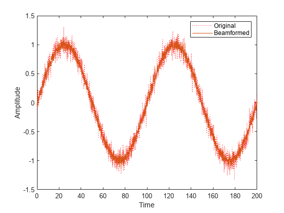
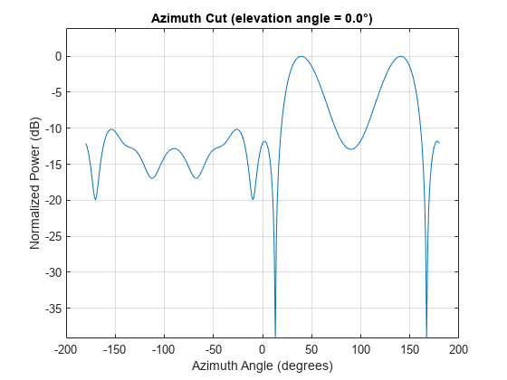
Apply an MVDR beamformer to a 5-element ULA. The incident angle of the signal is 45 degrees in azimuth and 0 degree in elevation. The signal frequency is .01 hertz. The carrier frequency is 300 MHz.

t = [0:.1:200]';
fr = .01;
xm = sin(2*pi*fr*t);
c = physconst('LightSpeed');
fc = 300e6;
rng('default');
incidentAngle = [45;0];
array = phased.ULA('NumElements',5,'ElementSpacing',0.5);
x = collectPlaneWave(array,xm,incidentAngle,fc,c);
noise = 0.1*(randn(size(x)) + 1j*randn(size(x)));
rx = x + noise;

Compute the beamforming weights.

beamformer = phased.MVDRBeamformer('SensorArray',array,...
    'PropagationSpeed',c,'OperatingFrequency',fc,...
    'Direction',incidentAngle,'WeightsOutputPort',true);
[y,w] = beamformer(rx);

Plot the signals.

plot(t,real(rx(:,3)),'r:',t,real(y))
xlabel('Time')
ylabel('Amplitude')
legend('Original','Beamformed')

Plot the array response pattern using the MVDR weights.

pattern(array,fc,[-180:180],0,'PropagationSpeed',c,...
    'Weights',w,'CoordinateSystem','rectangular',...
    'Type','powerdb');

Algorithms

MVDR Beamforming

The MVDR beamformer maximizes the signal to noise ratio.

Start with a signal arriving at the elements of an array. Assume that X is a complex-valued N-by-M data matrix representing the arrival of signals at an array. N is the number of sensors in the array and M is the number of samples or snapshots per signal. For mathematical convenience, this matrix is the transpose of the matrix specified in the X argument. Each row of X represents a time series of data for the corresponding array. The signal-to-noise ratio of a signal is given here.

$$SNR=\frac{{\left|w^{H}s\right|}^2}{w^H{R}_{I+N}^{}w}$$

Properly, the covariance matrix in the denominator is the covariance matrix for the noise and any interferers. You can vary the scale of w without affecting the SNR. Therefore, you can choose the normalization for w so that The MVDR estimator weights for beamforming are w = R^-1v/v^HRv where R is the data covariance matrix R = E[xx^H].

Diagonal Loading

Diagonal loading provides beamformer robustness due to small sample size and steering vector errors.

Data Precision

This System object supports single and double precision for input data, properties, and arguments. If the input data X is single precision, the output data is single precision. If the input data X is double precision, the output data is double precision. The precision of the output is independent of the precision of the properties and other arguments.

References

[1] Van Trees, H. Optimum Array Processing. New York: Wiley-Interscience, 2002.

[2] Frost, O. “An Algorithm For Linearly Constrained Adaptive Array Processing”, Proceedings of the IEEE. Vol. 60, Number 8, August, 1972, pp. 926–935.

Extended Capabilities

C/C++ Code Generation

Generate C and C++ code using MATLAB® Coder™.

Usage notes and limitations:

• See System Objects in MATLAB Code Generation (MATLAB Coder).

• This System object supports single and double precision for input data, properties, and arguments. If the input data X is single precision, the output data is single precision. If the input data X is double precision, the output data is double precision. The precision of the output is independent of the precision of the properties and other arguments.

Version History

Introduced in R2011a