clutterSurfaceRCS

Surface clutter radar cross section

Since R2021a

Syntax

rcs = clutterSurfaceRCS(nrcs,range,azimuth,elevation,graz,tau)

rcs = clutterSurfaceRCS(___,C)

rcs = clutterSurfaceRCS(___,Lp=beamshapeloss)

Description

rcs = clutterSurfaceRCS(nrcs,range,azimuth,elevation,graz,tau) returns the radar cross section, rcs, of the surface clutter patch.

rcs = clutterSurfaceRCS(___,C) returns the surface clutter radar cross-section with the propagation speed C.

rcs = clutterSurfaceRCS(___,Lp=beamshapeloss) returns the surface clutter radar cross-section using the beamshape loss.

Examples

Calculate Radar Cross Section (RCS) and Clutter to Noise Ratio (CNR)

Calculate the radar cross section of a clutter patch and estimate the clutter-to-noise ratio at the receiver. Assume that the patch is 1000 meters away from the radar system and the azimuth and elevation beamwidths are 1 degree and 3 degrees, respectively. Also assume that the grazing angle is 20 degrees, the pulse width is 10 microseconds, and the radar is operated at a wavelength of 1 cm with a peak power of 5 kw.

rng    = 1000;  
bwAz   = 1;     
bwEl   = 3;     
graz   = 20;    
tau    = 10e-6; 
lambda = 0.01; 
ppow   = 5000; 

Calculate the NRCS.

nrcs = landreflectivity('Mountains',graz)

nrcs = 
0.1082

Calculate clutter RCS using the calculated NRCS.

rcs = clutterSurfaceRCS(nrcs,rng,bwAz,bwEl,graz,tau)

rcs = 
288.9855

Calculate clutter-to-noise ratio using the calculated RCS.

cnr = radareqsnr(lambda,rng,ppow,tau,'rcs',rcs)

cnr = 
62.5974

RCS of Beam-Illuminated and Pulse-Illuminated Clutter

Since R2025a

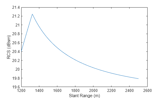
This example shows the RCS of the illuminated clutter region calculated as a function of slant range.

First, calculate the corresponding grazing angles for a set of ranges between 1.1 and 3 km. The radar is located at an altitude of 1 km and operates at a frequency of 1 GHz. It has a 5 degree symmetric beamwidth and a pulse width corresponding to 100 meters.

alt = 1e3;
freq = 1e9;
beamwidth = 5;
tau = 2*100/physconst('lightspeed');
slantRange = linspace(1.2e3,2.5e3,1e3).';
graze = asind(alt./slantRange);

Next, calculate surface NRCS using the Barton constant-gamma reflectivity model for farmland.

nrcs = landreflectivity('Farm',graze,freq);

Finally, calculate RCS and plot in dBsm. The inflection point around 1.3 km is caused by switching from the beam-limited clutter calculation to the pulse-limited clutter calculation.

rcs = clutterSurfaceRCS(nrcs,slantRange,beamwidth,beamwidth,graze,tau);
plot(slantRange,10*log10(rcs))
xlabel('Slant Range (m)')
ylabel('RCS (dBsm)')

Input Arguments

nrcs — Normalized radar cross section

nonnegative scalar | M-length vector of nonnegative values

Normalized radar cross section (NRCS) of a clutter patch specified as either a nonnegative scalar or an M-length vector of nonnegative values. Units are dimensionless but often expressed as m²/m². Each entry in nrcs corresponds to a slant range specified in range. The NRCS provides a measure of the reflectivity of a surface per unit area and is also referred to as σ⁰, the backscatter coefficient or reflectivity. NRCS can be determined from built-in surface models that are valid for pre-defined frequencies and grazing angles using landreflectivity and seareflectivity.

Example: nrcs = 1

Data Types: double

range — Clutter patch range (m)

nonnegative scalar | M-length vector of nonnegative values

Clutter patch slant range, specified as either a nonnegative scalar or an M-length vector of nonnegative values in units of meters. Each entry in range corresponds to a an entry in nrcs.

The Beam-Illuminated Approximation clutter approximation is valid at close range whereas the Pulse-Illuminated Approximation clutter approximation is valid at long range. See Beam-Limited and Pulse-Limited Clutter. (since R2025a)

Example: 1000

Data Types: double

azimuth — Azimuth beamwidth (deg)

positive scalar | [azimuth_Tx,azimuth_Rx]

Azimuth beamwidth of the radar, specified as a positive scalar or a 1-by-2 vector in units of degrees. Use with the elevation argument.

• When the transmit and receive beamwidths are the same, specify azimuth as a positive scalar.

• When the transmit and receive azimuth beamwidths are not the same, specify azimuth as a 1-by-2 positive vector [azimuth_Tx,azimuth_Rx], where the first element is the transmit azimuth beamwidth in degrees and the second element is the receive azimuth beamwidth.

clutterSurfaceRCS uses these two beamwidths to create an effective azimuth beamwidth. See Effective Beamwidth.

Example: 1

Data Types: double

elevation — Elevation beamwidth (deg)

positive scalar | [elevation_Tx,elevation_Rx]

Elevation beamwidth of the radar, specified as a positive scalar or a 1-by-2 vector in units of degrees. Use with the azimuth argument.

• When the transmit and receive beamwidths are the same, specify elevation as a positive scalar.

• When the transmit and receive elevation beamwidths are not the same, specify elevation as a 1-by-2 positive vector [elevation_Tx,elevation_Rx], where the first element is the transmit elevation beamwidth and the second element is the receive elevation beamwidth.

clutterSurfaceRCS uses these two beamwidths to create an effective elevation beamwidth. See Effective Beamwidth.

Example: 3

Data Types: double

graz — Grazing angle (deg)

nonnegative scalar | M-length vector of grazing values

Grazing angles of the clutter patches relative to the radar, specified as a nonnegative scalar or an M-length row vector of nonnegative values. Units are in degrees. Each entry in graz corresponds to a NRCS value specified in nrcs. See grazingang.

Data Types: double

tau — Pulse width (s)

nonnegative scalar

Pulse width of the transmitted signal, specified as a nonnegative scalar in units of seconds.

The pulse width is used to calculated the region illuminated by the radar for the Pulse-Illuminated Approximation approximation. (since R2025a)

Example: 10e-6

Data Types: double

C — Propagation speed (m/s)

speed of light (default) | positive scalar

Propagation speed, specified as a positive scalar in units of meters per second.

Data Types: double

beamshapeloss — Beamshape loss (dB)

0 dB (default) | nonnegative scalar

Beamshape loss, specified as a nonnegative scalar in decibels. The beamshape loss accounts for the reduced two-way antenna gain of off-axis scatterers.

Use this property when the elevation beamwidth (elevation) for the transmitter and receiver are not the same.

Example: Lp = 0

Data Types: double

Output Arguments

rcs — Radar cross section (m²)

scalar | M-length

The radar cross section of each surface clutter patch, returned as an scalar or M-length vector, in units of square meters.

More About

Effective Beamwidth

The effective beamwidth is used for the effective azimuth θ_azimutheff and effective elevation θ_elevationeff calculation when the transmitter and receiver beamwidths are not equal.

$$\begin{array}{l}{\theta }_{azimutheff}=\frac{\sqrt{2{\theta }_{at}{\theta }_{ar}}}{\sqrt{{\theta }_{at}{}^2+{\theta }_{ar}{}^2}}\\ {\theta }_{elvationeff}=\frac{\sqrt{2{\theta }_{et}{\theta }_{er}}}{\sqrt{{\theta }_{et}{}^2+{\theta }_{er}{}^2}}\end{array}$$

• at is the azimuth transmitter elevation beamwidth in degrees.

• ar is the azimuth receiver elevation beamwidth in degrees.

• et is the elevation transmitter elevation beamwidth in degrees.

• er is the elevation receiver elevation beamwidth in degrees.

Beam-Illuminated Approximation

At close range relevant to broadside pointing, clutterSurfaceRCS approximates the region illuminated by the radar as beam-illuminated. The extent of the beam-illuminated region depends on the radar beamwidth and the distance to the target. For a scenario geometry in which the radar beam is pointed downward so that it intersects a flat surface, the distance to the ground, or slant range, is a function of the radar altitude and grazing angle. Assume that the radar beam is conical with an elliptical beam footprint. The region illuminated by the beam is an ellipse defined by the intersection of the conical beam with the surface.

The area of the beam-illuminated region is approximated as a rectangle. The width, or extent in the azimuthal direction, W_beam, is taken as the arc length of the azimuth cut of the beam at the slant range, R. That is, $$W_{beam}=R{\theta }_{az}$$, where θ_az is the azimuth angle. This width is greater than the actual average width of the beam, but smaller than the maximum width of the beam. The length, or extent in the elevation direction, L_beam, is taken as the arc length of the elevation cut of the beam, modulated by the sine of the grazing angle, Ψ. That is, $$L_{beam}=\frac{R{\theta }_{el}}{\sin \Psi }$$, where θ_el is the elevation angle. This expression is applicable for broadside pointing and is most accurate for high grazing angles or short ranges. It may underestimate the true length of the region in other cases. The area of the beam-illuminated region, A_beam, is defined as A_beam = W_beam × L_beam.

Pulse-Illuminated Approximation

At long range, clutterSurfaceRCS approximates the region Illuminated by the radar as pulse-illuminated. The extent of the surface in the range direction that falls within one range bin is $$L_{pulse}=\frac{c\tau }{2\cos \Psi },$$ where $$\frac{c\tau }{2}$$ is the pulse width, $$\tau$$ (tau), given a propagation speed of c, and Ψ is the grazing angle. The figure below illustrates that the pulse width in the slant plane needs to be increased by a factor of $$\frac{1}{\cos \Psi }$$ to get the length of the pulse-illuminated region in the ground plane. The area of the pulse-illuminated region, A_pulse, is defined as A_pulse = W_beam* L_pulse.

Beam-Limited and Pulse-Limited Clutter

If the length of the pulse along the ground, L_pulse, is greater than the length of the beam-illuminated region, L_beam, then the illuminated region within a range cell has area A_beam. This is known as beam-limited clutter and tends to occur with high grazing angles. If L_pulse is less than L_beam, the area of the illuminated region is A_pulse. This is known as pulse-limited clutter and tends to occur for low grazing angles. The figure below shows these two regions as a function of grazing angle and pulse width for a scenario with a 1 km altitude and 5 degree azimuth and elevation beamwidths. Also see RCS of Beam-Illuminated and Pulse-Illuminated Clutter, which shows RCS as a function of slant range to highlight the inflection point that results from transitioning from a beam-limited to a pulse-limited clutter calculation.

References

[1] Barton, David K. Radar Equations for Modern Radar. Norwood, MA: Artech House, 2013.

[2] Long, Maurice W. Radar Reflectivity of Land and Sea. Boston: Artech House, 2001.

[3] Nathanson, Fred E., J. Patrick Reilly, and Marvin N. Cohen. Radar Design Principles. Mendham, NJ: SciTech Publishing, 1999.

Extended Capabilities

C/C++ Code Generation
Generate C and C++ code using MATLAB® Coder™.

Version History

Introduced in R2021a