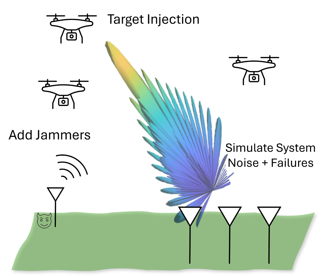
Augmenting Radar Data to Create More Diverse Datasets

Since R2025a

This example uses:

Introduction

Designing algorithms that are robust to noise and component failures is imperative for many applications. A wide variety of scenarios is often necessary to train machine learning and AI algorithms to achieve the highest levels of accuracy. In many instances, collecting data in challenging conditions, rare environments, or that include component failures is either impossible or too expensive. This example addresses these challenges and demonstrates how to model a range of conditions in the radar system by generating synthetic data and augmenting preexisting real data, including inserting synthetic targets into real data.

Motivation

In this example, we show how to augment both synthetic and real-world data with various target classes, noise sources, and component failures. This allows you to not only test your algorithms on challenging datasets but also to train on them. In the field of deep learning, data augmentation is a solution to the problem of limited data and encompasses a suite of techniques that enhance the size and quality of training datasets [1]. While many papers and programming libraries offer tools for augmenting computer vision data, few address the issue of augmenting radar data.

You might want to augment radar data for any of the following reasons:

Unbalanced Dataset: In collected data, certain target classes are less prevalent. Balance datasets by adding stochastic noise/errors to the data or by adding a copy of the target's response in other data recordings.
Avoid Overfitting: Modify generated or synthetic data to train or test algorithms on similar but different radar data cubes to improve a model's capability to generalize.
Simulate Rare or Expensive Conditions/Settings: Create synthetic data or modify already collected data to model scenarios that are difficult to achieve with actual hardware.
Define Critical Thresholds: Investigate stressors like how much antenna phase noise is too much or how many antenna failures before a system can no longer operate well enough.

Synthetic Data Generation and Augmentation

No Modification or Augmentation

Create a Digital Twin of a TI mmWave Radar demonstrates how to model a real-world radar system using radarTransceiver and establishes that simulated data is similar to real data collected with the actual radar. Just as in that example, create a radarTransceiver along with the necessary processing steps for the Texas Instruments' (TI) IWR1642BOOST automotive radar. This section generates synthetic data with a constant velocity point target. Because there is no target acceleration or requirement to update the trajectory between chirps, set the radar transceiver's number of repetitions property to the number of chirps in a coherent processing interval.

addpath("tiRadar")
rng('default')
radarCfg = helperParseRadarConfig("config_Fri_11_1.cfg");
radarSystem = helperRadarAndProcessor(radarCfg);
radarSystem.RadarTransceiver.NumRepetitions = radarCfg.NumChirps; % Use with target that does not need manual move/update between chirps

Next, create a target and plot its range-Doppler response. Before computing the range-Doppler response, first reformat the data such that there are 8 (virtual) channels instead of 4. Then, sum across the channel dimension to beamform towards boresight. Finally compute the range-Doppler response on the beamformed data. Execute this beamforming and range-Doppler response using the boresightRD method below.

tgt = struct('Position', [7 3 0], 'Velocity', [1.5 .5 0],'Signatures',{rcsSignature(Pattern=15)});
time = 0;
sigOriginalSynth = radarSystem.RadarTransceiver(tgt,time);
sigOriginalSynth = radarSystem.downsampleIF(sigOriginalSynth);
[rgdpOrignal,rngBins,dpBins] = radarSystem.boresightRD(sigOriginalSynth);

Find the maximum value in the range-Doppler response and set that as the peak location. Use this location as the bin of interest for the next synthetic data section as well.

[~,I] = max(rgdpOrignal,[],"all");
[rangePeakIdx,dopPeakIdx] = ind2sub(size(rgdpOrignal),I);

helperPlotRangeDoppler(rgdpOrignal,rngBins,dpBins,rangePeakIdx,dopPeakIdx,'Original Synthetic Data Range-Doppler');

Figure contains an axes object. The axes object with title Original Synthetic Data Range-Doppler, xlabel Range (m), ylabel Doppler (m/s) contains 2 objects of type image, scatter. This object represents Target Peak Bin.

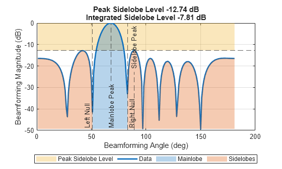
Next, perform phase shift beamforming on that detected range-Doppler bin using the helper getBfRangeAnglePatch method. As explained in Create a Digital Twin of a TI mmWave Radar, the helper class implements a correction for target motion since the TI radar uses time-division multiplexing (TDM). Then, plot the beamforming output along with a visualization of its peak and integrated sidelobe levels using sidelobelevel.

bfOutOriginal = radarSystem.getBfRangeAnglePatch(sigOriginalSynth,[rangePeakIdx;dopPeakIdx],rngBins,true);
sidelobelevel(mag2db(abs(bfOutOriginal)))
xlabel('Beamforming Angle (deg)')
ylabel('Beamforming Magnitude (dB)')

Figure contains an object of type phased.internal.sidelobelevelchart.

Antenna Noise

One way to modify synthetic radar data is to manipulate the antenna elements of the radar. Beyond specifying the antenna elements' directivity pattern, one can also model array perturbations as shown in Modeling Perturbations and Element Failures in a Sensor Array. Synthesizing data with these antenna perturbations offers an explainable insertion of system noise that can be processed properly in the transmitter and receiver architecture. These perturbations can account for the following phenomena:

Miscalibration or changing calibration
Antenna position errors caused by vibration or device damage
Elements Failures
Antenna corrosion

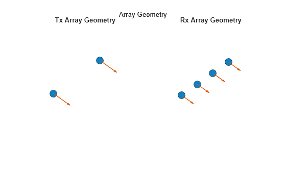
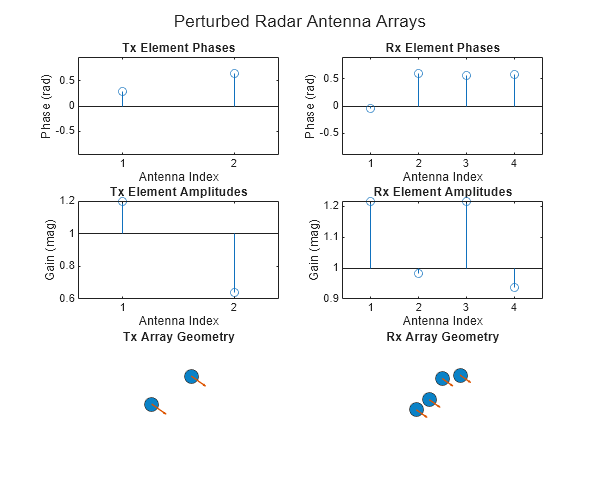
The TI radar modeled here has a transmit antenna array with two antennas spaced two wavelengths apart and a receive antenna array with four antennas each spaced a half of a wavelength apart.

figure;
subplot(1,2,1)
viewArray(radarSystem.RadarTransceiver.TransmitAntenna.Sensor,'ShowLocalCoordinates',false,'ShowAnnotation',false,'ShowNormals',true)
title('Tx Array Geometry')
subplot(1,2,2)
viewArray(radarSystem.RadarTransceiver.ReceiveAntenna.Sensor,'ShowLocalCoordinates',false,'ShowAnnotation',false,'ShowNormals',true)
title('Rx Array Geometry')

Figure contains 2 axes objects. Hidden axes object 1 with title Tx Array Geometry contains 2 objects of type scatter, quiver. Hidden axes object 2 with title Rx Array Geometry contains 2 objects of type scatter, quiver.

Using TDM, the transmit and receive antenna arrays manifest into the following virtual array.

figure;
viewArray(radarSystem.VirtualArray)
title('Virtual Array')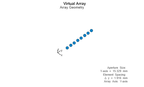

Figure contains an axes object. The hidden axes object with title Virtual Array, xlabel x axis (Az 0 El 0) -->, ylabel y axis --> contains 7 objects of type scatter, line, text.

Add gaussian noise to the phase and amplitude of each antenna and position error by setting the standard deviation of the added noise for each perturbation. In this example, the phase noise and position noise are zero-mean while the amplitude noise has a mean of one. Create a custom struct antennaNoiseCfg with properties AntennaPhaseNoiseSTD, AntennaAmplitudeNoiseSTD, and AntennaPositionNoiseSTD to enable the antenna perturbations and set the standard deviations for each.

antennaNoiseCfg.AntennaPhaseNoiseSTD              = 0.4;

antennaNoiseCfg.AntennaAmplitudeNoiseSTD          = 0.3;

lambda = freq2wavelen(radarSystem.Fc);
antennaNoiseCfg.AntennaPositionNoiseSTD = lambda * 0.06;
radarSystemPerturbed = helperRadarAndProcessor(radarCfg,antennaNoiseCfg);
radarSystemPerturbed.RadarTransceiver.NumRepetitions = radarCfg.NumChirps;

helperPlotAntennaPerturbations(radarSystemPerturbed.RadarTransceiver)
sgtitle('Perturbed Radar Antenna Arrays')

Now, with the perturbed antenna arrays, plot the range-Doppler and beamforming outputs. Notice the worsening of the sidelobe level in the beamforming output compared with the unperturbed radar system.

sig = radarSystemPerturbed.RadarTransceiver(tgt,time);
sig = radarSystem.downsampleIF(sig);

rgdp = radarSystemPerturbed.boresightRD(sig);
bfOut = radarSystemPerturbed.getBfRangeAnglePatch(sig,[rangePeakIdx;dopPeakIdx],rngBins,true);

helperPlotRangeDoppler(rgdp,rngBins,dpBins,rangePeakIdx,dopPeakIdx,'Perturbed Array Synthetic Data Range-Doppler');

Figure contains an axes object. The axes object with title Perturbed Array Synthetic Data Range-Doppler, xlabel Range (m), ylabel Doppler (m/s) contains 2 objects of type image, scatter. This object represents Target Peak Bin.

f = figure;
f.Position(3:4) = [500 500];
sidelobeLevelPlot = tiledlayout(2,1);
sidelobelevel(mag2db(abs(bfOutOriginal)),'Parent',sidelobeLevelPlot)
xlabel('Beamforming Angle (deg)')
ylabel('Beamforming Magnitude (dB)')

nexttile
sidelobelevel(mag2db(abs(bfOut)),'Parent',sidelobeLevelPlot)
xlabel('Beamforming Angle (deg)')
ylabel('Beamforming Magnitude (dB)')
sidelobeLevelPlot.Title.String ={'Beamforming Comparison','Without (Top) and With (Bottom) Perturbation'};

Figure contains objects of type phased.internal.sidelobelevelchart.

Augment Real Collected Data

Many times, data augmentation involves taking already collected and even labeled data and modifying it to increase the size and variety of the dataset. The following sections demonstrate multiple ways that you can easily augment already collected data. First, load in a collected data file filled with radar data from the IWR1642BOOST. In the recorded data, a person walks around holding a corner reflector. The human and corner reflector imitate a moving point target.

% load in data
frames = load('humanAndCorner.mat').humanAndCorner;

Here, a frame refers to a single coherent processing interval, or CPI. Each frame/CPI has its own data cube. Each data cube is formatted such that the dimensions are (in order), samples per chirp, number of channels, and number of chirps. The chirps have already been arranged so that there are eight channels for every chirp based on the TDM configuration.

frameSize = size(frames(:,:,:,1))

frameSize = 1×3

   256     8    16

nFrame = size(frames,4)

nFrame = 
25

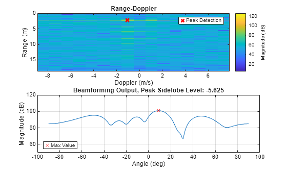
Compute and display the range-Doppler response and beamforming output of the original collected data below. The removeClutter flag subtracts the mean chirp of each frame, which reduces the reflected power of static objects.

removeClutter = true;
f = figure;
pslArrayOriginal = [];
for frameIdx = 1:nFrame
    sig = frames(:,:,:,frameIdx);
    if removeClutter
        sig = sig - mean(sig,3);
    end
    [psl,realDataMaxRD] = helperRangeDopplerAngle(sig,radarSystem,f);
    pslArrayOriginal = [pslArrayOriginal; psl]; %#ok<AGROW>
    pause(.1)
end

Antenna Phase and Gain

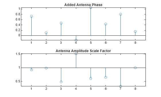
You can introduce noise in the amplitude and phase of the virtual antenna arrays just as we did in the simulated radarTransceiver above. A number of real world phenomena can cause these changes in amplitude and phase including miscalibration, interference, and antenna position errors. You can account for these errors by adding a gain and phase to each of the channels in the collected signal. The amplitude and phase errors across the elements of the virtual array are the combination of the amplitude and phase errors on the elements of the receive and transmit arrays. To simulate phase and gain noise in both the transmit and receive signal, sample six normally distributed distributions, one for each antenna.

std = 0.6;
phases = exp(1j*std*randn(1,6,1));

std = 0.2;
amps = ones([1,6,1]) + std*randn(1,6,1);

Let the first two values in the phase and magnitude vectors belong to the transmit antenna array and the rest belong to the receive antenna array. Then, multiply the phases and gains together such that the phase and gain of each transmit antenna is distributed over all four receive antenna values. Lastly, multiple the phase and gain values together.

% length is 8 because of virtual array size
phase2add = [phases(1)*phases(3:end), phases(2)*phases(3:end)];
amp2add = [amps(1)*amps(3:end), amps(2)*amps(3:end)]; 
antennaPerturbation = amp2add .* phase2add;

Plot the virtual antenna perturbations below.

figure;
subplot(2,1,1)
stem(angle(antennaPerturbation))
title('Added Antenna Phase')
subplot(2,1,2)
stem(abs(antennaPerturbation),'BaseValue',1)
title('Antenna Amplitude Scale Factor')

Figure contains 2 axes objects. Axes object 1 with title Added Antenna Phase contains an object of type stem. Axes object 2 with title Antenna Amplitude Scale Factor contains an object of type stem.

Now with the perturbed antennas, process and display the radar data.

removeClutter = true;
f = figure;
pslArray = [];
for frameIdx = 1:nFrame
    sig = frames(:,:,:,frameIdx);
    if removeClutter
        sig = sig - mean(sig,3);
    end
    sig = antennaPerturbation .* sig;
    psl = helperRangeDopplerAngle(sig,radarSystem,f);
    pslArray = [pslArray; psl]; %#ok<AGROW>
    pause(.1)
end

Compare the peak sidelobe level (PSL) for the beamforming output with and without the antenna perturbations for each frame.

figure;
plot(pslArrayOriginal,'LineWidth',2)
hold on
plot(pslArray,'LineWidth',2)
fill([1:nFrame,nFrame:-1:1], [pslArrayOriginal; flipud(pslArray)], 'r','FaceAlpha',0.1,'EdgeColor','none');
legend({'PSL Original','PSL With Added Noise','PSL Loss'},'Location','southoutside')
title({'Peak Sidelobe Level Comparison','(Lower Value is Better)'})
xlabel('Frame/CPI Index')
ylabel('PSL (dB)')

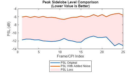
Figure contains an axes object. The axes object with title Peak Sidelobe Level Comparison (Lower Value is Better), xlabel Frame/CPI Index, ylabel PSL (dB) contains 3 objects of type line, patch. These objects represent PSL Original, PSL With Added Noise, PSL Loss.

You can see in the plot above that the peak sidelobe level is worsened when phase and gain measurements are added to the collected radar data.

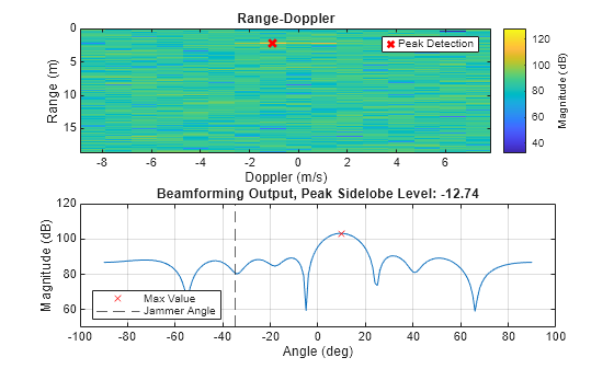
Add a Barrage Jammer

In addition to modifying the radar system, you can also modify the radar environment in a number of ways. For example, add a barrage jammer. Define a barrage jammer with an effective radiated power of one megawatt. Then place the jammer at an azimuth using the slider below. Generate a steering vector to reflect the location of the jammer using the fact that the virtual antenna array elements are each a half a wavelength apart.

jammer = barrageJammer('ERP',1e6,'SamplesPerFrame',size(sig,1)*size(sig,3));
jammerAngle = -35; % deg
jamSteerer = steervec(.5*(0:7),jammerAngle);

For each frame, plot the range-Doppler response and beamforming output. The plots below show an elevated noise floor that makes it harder to detect the target consistently. Furthermore, when the jammer overtakes the target in power, we see the beamforming peak at the same azimuth angle as the jammer.

removeClutter = true;
f = figure;
pslArray = [];
for frameIdx = 1:nFrame
    sig = frames(:,:,:,frameIdx);
    if removeClutter
        sig = sig - mean(sig,3);
    end
    jamSig = jammer();
    jamSig = reshape(jamSig,[size(sig,1),1,size(sig,3)]);
    jamSig = repmat(jamSig,1,8,1);
    jamSig = jamSig.*reshape(jamSteerer,[1,8,1]);
    sig = sig + jamSig;
    psl = helperRangeDopplerAngle(sig,radarSystem,f,jammerAngle,'Jammer Angle');
    pslArray = [pslArray; psl]; %#ok<AGROW>
    pause(.1)
end

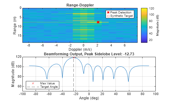
Insert a Synthetic Target (Target Injection)

You can also add synthetic targets to real data. Use the synthetic target from the beginning of this example. When inserting a synthetic target, you do not want to inadvertently add synthetic noise to the real signal. To avoid this, remove the noise in the LNA and then regenerate the raw signal with the target reflection.

release(radarSystem.RadarTransceiver.Receiver.Cascade{1})
radarSystem.RadarTransceiver.Receiver.Cascade{1}.IncludeNoise = false;
sigSynthNoNoise = radarSystem.RadarTransceiver(tgt,time);
sigSynthNoNoise = radarSystem.downsampleIF(sigSynthNoNoise);

Plot the range-Doppler response of the noise-free signal.

rgdpSynthNoNoise = radarSystem.boresightRD(sigSynthNoNoise);
helperPlotRangeDoppler(rgdpSynthNoNoise,rngBins,dpBins,rangePeakIdx,dopPeakIdx,'Noise-Free Synthetic Data Range-Doppler');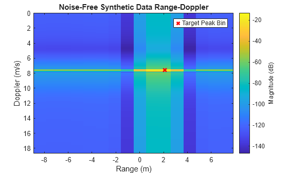

Figure contains an axes object. The axes object with title Noise-Free Synthetic Data Range-Doppler, xlabel Range (m), ylabel Doppler (m/s) contains 2 objects of type image, scatter. This object represents Target Peak Bin.

Then, reformat the synthetic signal so that it has eight virtual channels in its channel dimension. Do this by concatenating pairs of consecutive chirps.

targetVirt = cat(2,sigSynthNoNoise(:,:,1:2:end),sigSynthNoNoise(:,:,2:2:end));

Next, scale the magnitude of the noise-free target signal to achieve the desired SNR, probability of detection, radar cross section, received power, or any other desired metric. For this example, set the single pulse received power to -8 dB by scaling the synthetic signal appropriately.

desiredPulsePowerdB = -8;
desiredPulsePowerWatts = db2pow(desiredPulsePowerdB);
originalPulsePowerWatts = rms(targetVirt(:,1,1))^2;
targetVirt = desiredPulsePowerWatts * targetVirt/originalPulsePowerWatts;

Afterwards, load in a new recording of real data into which the synthetic target will be injected.

% Load the new clutter environment
frames = load('newClutterNoTarget.mat').newClutterNoTarget;
nFrame = size(frames,4);

Lastly, for each frame, add the synthetic target signal to the real data and then plot the range-Doppler response and beamforming output.

targetAngle = -atand(tgt.Position(2)/tgt.Position(1));
% Process and plot the data
f = figure;
for frameIdx = 1:nFrame
    sig = frames(:,:,:,frameIdx);
    sig = sig+targetVirt;
    psl = helperRangeDopplerAngle(sig,radarSystem,f,targetAngle,'Target Angle');
    set(0,'CurrentFigure',f)
    subplot(2,1,1)
    plot(dpBins(dopPeakIdx),rngBins(rangePeakIdx),'rs','DisplayName','Synthetic Target')
    pause(.5)
end

Summary

This example shows how to augment both synthetic and real data and demonstrates ways to introduce phase and magnitude errors, jammers, and synthetic targets. With these tools, you can augment radar datasets to include more variety as well as rare or expensive scenarios that would be hard to collect in real life. The skills and tools demonstrated in this example can be extrapolated to include different sources of noise as well as other failures for your workflows.

References

[1] Shorten, Connor, and Taghi M. Khoshgoftaar. "A survey on image data augmentation for deep learning." Journal of big data 6, no. 1 (2019): 1-48.

Helper Functions

function dataOut = helperReformatData(dataIn)
    % put it in format such that there are only 4 channels and the chirps
    % are from alternating transmitters     
    dataOut = zeros(size(dataIn,1),.5*size(dataIn,2),2*size(dataIn,3));
    dataOut(:,:,1:2:end) = dataIn(:,1:4,:);
    dataOut(:,:,2:2:end) = dataIn(:,5:end,:);
end

%% Plotting Helper Functions

function helperPlotRangeDoppler(rgdp,rngBins,dpBins,rangePeakIdx,dopPeakIdx,titleStr)
    rgdp = mag2db(abs(rgdp));

    figure;
    imagesc(dpBins, rngBins, rgdp)
    hold on
    scatter(dpBins(dopPeakIdx),rngBins(rangePeakIdx),50,'rx','LineWidth',2)
    legend('Target Peak Bin')
    xlabel('Range (m)')
    ylabel('Doppler (m/s)')
    title(titleStr)
    c = colorbar;
    c.Label.String = 'Magnitude (dB)';
end


function helperPlotAntennaPerturbations(xcvr)
    txArray = xcvr.TransmitAntenna.Sensor;
    rxArray = xcvr.ReceiveAntenna.Sensor;
    
    txAngle = angle(txArray.Taper);
    rxAngle = angle(rxArray.Taper);
    
    txAmp = abs(txArray.Taper);
    rxAmp = abs(rxArray.Taper);
    
    f = figure;
    f.Position(3:4) = [600 500];
    subplot(3,2,1)
    stem(txAngle)
    xticks([1,2])
    ylim(max(abs(txAngle))*[-1.5 1.5])
    title('Tx Element Phases')
    xlabel('Antenna Index')
    ylabel('Phase (rad)')
    subplot(3,2,2)
    stem(rxAngle)
    ylim(max(abs(rxAngle))*[-1.5 1.5])
    title('Rx Element Phases')
    xlabel('Antenna Index')
    ylabel('Phase (rad)')
    
    subplot(3,2,3)
    stem(txAmp,'BaseValue',1)
    xticks([1,2])
    title('Tx Element Amplitudes')
    xlabel('Antenna Index')
    ylabel('Gain (mag)')
    subplot(3,2,4)
    stem(rxAmp,'BaseValue',1)
    title('Rx Element Amplitudes')
    xlabel('Antenna Index')
    ylabel('Gain (mag)')
    
    subplot(3,2,5)
    viewArray(txArray,'ShowLocalCoordinates',false,'ShowAnnotation',false,'ShowNormals',true,'Title','');
    title('Tx Array Geometry')
    subplot(3,2,6)
    viewArray(rxArray,'ShowLocalCoordinates',false,'ShowAnnotation',false,'ShowNormals',true,'Title','');
    title('Rx Array Geometry')
    
end

function [psl,maxRD] = helperRangeDopplerAngle(sig,radarSystem,fig,optionalXLine,optionalXlineName)
    rgdp = zeros(size(sig));
    for channelIdx = 1:8
        [rgdp(:,channelIdx,:),rngBins,dpBins] = radarSystem.RangeDopplerProcessor(squeeze(sig(:,channelIdx,:)));
    end
    
    % Find Max Range Doppler Bin (Simple Detector)
    rgdpSumChannels = squeeze(sum(rgdp,2)); % beamform toward boresight
    [~,I] = max(abs(rgdpSumChannels),[],'all');
    [rangePeakIdx,dopPeakIdx] = ind2sub(size(rgdpSumChannels),I);
    
    sig = helperReformatData(sig);
    bfOut = radarSystem.getBfRangeAnglePatch(sig,[rangePeakIdx;dopPeakIdx],rngBins,true);
    bfOut = mag2db(abs(bfOut));
    psl=sidelobelevel(bfOut);
    
    set(0,'CurrentFigure',fig)
    
    subplot(2,1,1)
    imagesc(dpBins,rngBins,mag2db(abs(rgdpSumChannels)))
    hold on;
    scatter(dpBins(dopPeakIdx),rngBins(rangePeakIdx),50,'rx','LineWidth',2)
    xlabel('Doppler (m/s)')
    ylabel('Range (m)')
    title('Range-Doppler')
    legend('Peak Detection')
    c = colorbar;
    c.Label.String = 'Magnitude (dB)';

    sp2 = subplot(2,1,2);
    cla(sp2,'reset');
    angles = -90:90;
    plot(angles,bfOut,'HandleVisibility','off');
    [maxRD,I] = max(bfOut);
    hold on
    plot(angles(I),maxRD,'rx','DisplayName','Max Value')
    ylim([50,120])
    title(['Beamforming Output, Peak Sidelobe Level: ' num2str(psl,4)])
    xlabel('Angle (deg)')
    ylabel('Magnitude (dB)')
    if exist('optionalXLine','var') && exist('optionalXlineName','var')
        xline(optionalXLine,'--','DisplayName',optionalXlineName)
    end
    grid on
    
    legend('Location','southwest')
end