I/Q Data Collection and Detection Generation with Texas Instruments (TI) millimeter-wave (mmWave) Radar

Since R2024b

This example serves as an introduction to analyzing real-world radar I/Q data captured using the TI mmWave Radar Sensors Hardware Support Package (HSP). With this HSP and lessons from this tutorial, you can develop advanced radar signal processing applications using real-world I/Q data in MATLAB®.

Introduction

Radar Toolbox™ allows you to collect I/Q data from the TI mmWave radar sensor family. This example is designed to introduce you to the process of capturing and analyzing real-world I/Q data in MATLAB®.

To illustrate a typical development workflow, we analyze the range, Doppler, and angle responses of the radar board with a single target at a known range, speed and off-boresight angle. With this information in mind, we develop a simple detection generation algorithm geared towards people detection.

The example is structured to provide you with a practical understanding of the signal processing workflow, including data visualization. Importantly, this example can run using recorded data, or through direct streaming for those with access to a TI radar board and a data acquisition board (DCA1000EVM).

It's worth noting that Radar Toolbox™ can also be used to collect detection point clouds from TI mmWave radars as opposed to raw I/Q data. The ability to collect raw I/Q data not only broadens the scope of potential applications but also deepens the understanding of the underlying signal processing techniques. For more information on using the detection point cloud outputs from the TI radars, see People Tracking Using TI mmWave Radar (Sensor Fusion and Tracking Toolbox) and Track Objects in a Parking Lot Using TI mmWave Radar (Sensor Fusion and Tracking Toolbox).

Data Collection

A pre-recorded set of data is used to run this example. The following code downloads the required data files into the current working directory if it is not already present. This downloaded data is used for the remainder of the example.

% Load and unzip data if unavailable. 
if ~exist('TIRadarIntroIQData','dir')
    dataURL = "https://ssd.mathworks.com/supportfiles/timmwaveradar/data/TIRadarIntroIQData.zip";
    datasetFolder = pwd;
    unzip(dataURL, datasetFolder);
end

% Data file path
dataFilePath = fullfile(pwd,'TIRadarIntroIQData','ExampleIQData.mat');

% Video file path
videoFilePath = fullfile(pwd,'TIRadarIntroIQData','ExampleVideoData.mp4');

The function helperDataCollectionProcedure was run to collect all of the data that is used to generate the figures in this example. This function is included as a separate file with this example. In order to rerun the data collection procedure, run the following function.

helperDataCollectionProcedure('IWR1642BOOST');

System Overview

Hardware Setup

In order to collect I/Q data from a TI mmWave radar, two pieces of hardware are required:

1. The TI mmWave radar evaluation module. This board generates and transmits the radar waveform from an array of transmit antennas and captures the reflected waveforms from an array of receive antennas, mixing the received waveform with the transmitted waveform to generate the intermediate frequency (IF).

2. The DCA1000 evaluation module for real-time data capture. This board digitally samples the waveforms received by the radar board.

We used the IWR1642BOOST model to collect data for this example, but there are a number of supported radar boards. This list can be found on the TI mmWave Radar Sensors page.

model = 'IWR1642BOOST';

Radar Waveform

The waveform transmitted by the TI mmWave radar is a linear Frequency Modulated Continuous Wave (FMCW) chirp. These waveforms are ubiquitous in modern radar technology and a number of examples have investigated FMCW processing and will therefore will not be discussed in detail as part of this example. For more information on FMCW signal processing, see Automotive Adaptive Cruise Control Using FMCW Technology.

One important point to mention is that although an FMCW waveform is transmitted by the radar, as is typical with these systems, the received signal is mixed with the transmitted signal in the radar receiver. This means that the data sampled by the DCA1000 and collected in this example is the already dechirped intermediate frequency (IF) data. Therefore, in order to determine the range response from the data, we simply need to take the Discrete Fourier Transform (DFT) of the collected data. The ranges of the targets in the scene are directly proportional to the beat frequencies observed after taking the DFT.

Radar Board Configuration

The radar in this example is configured for people detection. The radar configuration is specified in a separate file when the object is created. Many of the operating parameters of the radar are tunable including but not limited to the sweep bandwidth, sweep slope, sweep duration, pulse repetition frequency (PRF), number of chirps, and transmission pattern. These parameters can be modified to meet the operating requirements of the radar. For more information on configuring the radar, see the TI mmWave Radar Sensors documentation page.

In this example we configured the radar to function for people detection. Specifically, we had the following operating requirements:

• The radar should be able to detect people in a large room, so the maximum unambiguous range should be >15 m.

• The radar should be able to detect people moving at walking speeds, so the maximum unambiguous velocity should be >2 m/s.

• The range resolution should be <0.1 m.

• The velocity resolution should be <0.15 m/s.

reqMaxRange = 15;
reqRangeResolution = 0.1;
reqMaxVelocity = 2;
reqVelocityResolution = 0.15;

We saved the configuration of the radar that was used for data collection in a helper class included with this example. We can load the configuration from the attached data file by running the following command.

load(dataFilePath,'radarConfiguration');

By saving the configuration that was used for data collected, we are able to verify that the radar as configured meets the operating requirements defined above. Additionally, this radar configuration gives us access to a number of properties that were configured at the time of data collection (e.g. sweep slope, sweep time, number of chirps, etc.) which will allow us to effectively analyze the collected data in later parts of this example. The radar configuration at the time of data collection is displayed below.

disp(radarConfiguration);

  helperRadarConfiguration with properties:

         StartFrequency: '77 (GHz)'
          StopFrequency: '78.775 (GHz)'
        CenterFrequency: '77.975 (GHz)'
              Bandwidth: '1.6 (GHz)'
               RampTime: '75 (us)'
         ChirpCycleTime: '225 (us)'
             SweepSlope: '25 (MHz/us)'
        SamplesPerChirp: 400
          ADCSampleRate: '6250 (ksps)'
              NumChirps: 80
           NumReceivers: 4
        ActiveReceivers: [1 1 1 1]
        NumTransmitters: 2
     ActiveTransmitters: [1 1]
       FramePeriodicity: '100 (ms)'
           MaximumRange: '37.4741 (m)'
        RangeResolution: '0.093685 (m)'
      AzimuthResolution: '14.4775 (degrees)'
       MaximumRangeRate: '2.136 (m/s)'
    RangeRateResolution: '0.1068 (m/s)'

The radar configuration conveniently includes the performance requirements that we are interested in. The table below shows that the radar is configured such that it will meet our operating requirements.

Requirements = ["Max Unambiguous Range";"Range Resolution";"Max Unambiguous Velocity";"Velocity Resolution"];
Objective = [reqMaxRange;reqRangeResolution;reqMaxVelocity;reqVelocityResolution];
Actual = [radarConfiguration.MaximumRange/2;radarConfiguration.RangeResolution;radarConfiguration.MaximumRangeRate;radarConfiguration.RangeRateResolution];
reqTable = table(Requirements,Objective,Actual);
disp(reqTable);

           Requirements           Objective     Actual 
    __________________________    _________    ________

    "Max Unambiguous Range"           15         18.737
    "Range Resolution"               0.1       0.093685
    "Max Unambiguous Velocity"         2          2.136
    "Velocity Resolution"           0.15         0.1068

Antenna Geometry

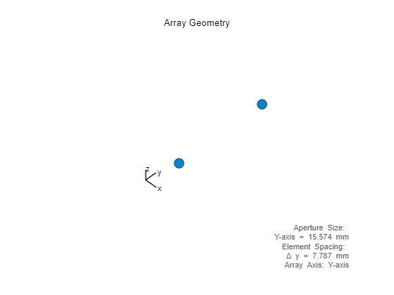
The IWR1642BOOST evaluation board that is used for this example contains two transmit elements and four receive elements.

The transmit elements are arranged as a uniform linear array (ULA) with two wavelength spacing.

lambda = freq2wavelen(77e9);
txArray = phased.ULA(NumElements=2,ElementSpacing=2*lambda);
figure;
viewArray(txArray);

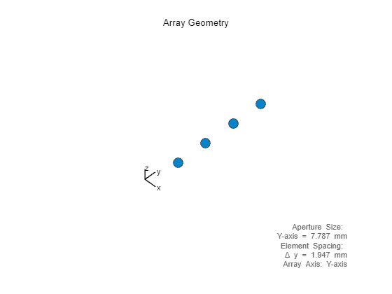
The receive elements are arranged as a ULA with half wavelength spacing.

rxArray = phased.ULA(NumElements=4,ElementSpacing=lambda/2);
figure;
viewArray(rxArray);

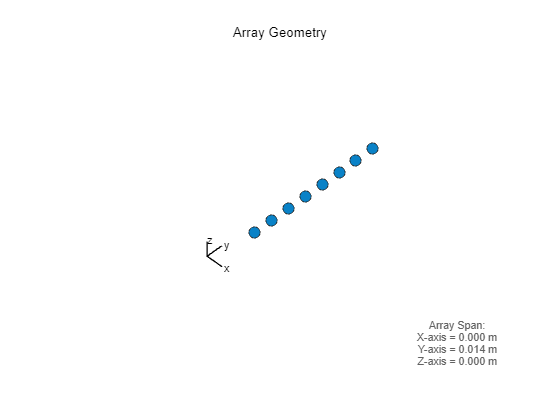
The radar is configured to operate using Time Division Multiplexing (TDM). This means that transmissions alternate between the first and second transmit antenna. By grouping these alternating transmissions together, we can create an eight-element virtual array with half lambda spacing, giving us finer angular resolution than would normally be achieved with a four-element receive array. For more information on virtual arrays, see Increasing Angular Resolution with Virtual Arrays.

The following code shows how to create a virtual array based on the transmitter and receiver positions using a phased.ConformalArray. The geometry of the virtual array being used in this example is a ULA.

nTx = radarConfiguration.NumTransmitters;
txPos = getElementPosition(txArray);
nRx = radarConfiguration.NumReceivers;
rxPos = getElementPosition(rxArray);
virtualPos = zeros(3,nTx*nRx);
for iTx = 0:nTx-1
    startIdx = iTx*nRx+1;
    endIdx = startIdx+nRx-1;
    virtualPos(:,startIdx:endIdx) = rxPos + txPos(:,iTx+1);
end
virtualArray = phased.ConformalArray(ElementPosition=virtualPos);
figure;
viewArray(virtualArray);

The data that is collected from the radar is arranged into pulse groups that alternate between the two active transmitters. This means that the data has to be rearranged after collection to the expected dimensions for the virtual array. The size of the data initially has the dimensions of the number of data samples by the number of receivers by the number of chirps, but the chirps switch off between active transmissions.

load(dataFilePath,'dataSnapshot');
disp(size(dataSnapshot));

   400     4    80

The code below shows how we can rearrange a data snapshot depending on the number of active transmitters into the correct configuration for processing the virtual array data cube. By rearranging the data in this fashion, we are making the simplifying assumption that each alternating transmission is happening at the same time. By doing so, we double the number of spatial channels while halving the number of slow time chirps.

nSamples = radarConfiguration.SamplesPerChirp;
nChirps = radarConfiguration.NumChirps;
virtualData = zeros(nSamples,nRx*nTx,nChirps/nTx);
for iTx = 0:nTx-1
    startIdx = iTx*nRx+1;
    endIdx = startIdx+nRx-1;
    virtualData(:,startIdx:endIdx,:) = dataSnapshot(:,:,iTx+1:nTx:end);
end
disp(size(virtualData));

   400     8    40

This approach for rearranging the data into a virtual data cube is applied for the remainder of the example.

I/Q Data Analysis

The first part of this example looks at the properties of the I/Q data that is generated by a TI mmWave radar when a single target is present at known locations, speeds and angles. This analysis helps inform our development of the detection generation algorithm in the second part of the example.

Range-Doppler Response

To investigate the range-Doppler response of the radar, data is collected in two controlled setups:

1. A single stationary corner reflector is placed 2 meters from the radar at boresight.

2. A single corner reflector is held in someone's hand as they walk towards the radar at ~1 mph (~0.5 m/s).

In this section we analyze the range-Doppler response of both setups to see whether the results match our expectations and whether it would be beneficial to use a windowing function for range and Doppler processing.

Single Stationary Reflector

First, we load the data snapshot collected with a single stationary corner reflector. We load the data cube and rearrange it into the correct dimensions for the virtual array using helperArrangeVirtualData as discussed in Antenna Geometry.

load(dataFilePath,'stationaryReflectorData');
stationaryReflectorData = helperArrangeVirtualData(stationaryReflectorData,radarConfiguration);

In order to process the range-Doppler response, we first extract some key information from the radar configuration. Note that in TDM, the time between chirps for a single virtual receiver is the product of the chirp cycle time and the number of transmitters, due to the alternating transmissions. This fact is reflected in the calculation of the PRF.

% Sampling rate (Samples/s)
fs = radarConfiguration.ADCSampleRate*1e3;

% Sweep slope (Hz/s)
sweepSlope = radarConfiguration.SweepSlope*1e6/1e-6;

% Center frequency (Hz)
fc = radarConfiguration.CenterFrequency*1e9;

% PRF (Hz)
prf = 1e6/(radarConfiguration.NumTransmitters*radarConfiguration.ChirpCycleTime);

A phased.RangeDopplerResponse object is created to assist with range-Doppler processing and visualization. We configure the object using the operating parameters defined above. Note that the RangeMethod is set to FFT. This is because the data sampled by the DCA1000 was already dechirped on the TI mmWave radar board as discussed in the Radar Waveform section.

rdResponse = phased.RangeDopplerResponse(RangeMethod="FFT",...
    DechirpInput=false,SampleRate=fs,SweepSlope=sweepSlope,...
    DopplerOutput='Speed',OperatingFrequency=fc,PRFSource='Property',...
    PRF=prf);

We plot the range-Doppler response image using the plotResponse method for data captured by the first antenna element. We visualize the area from 0 to 5 meters to make it easier to see.

figure;
plotResponse(rdResponse,squeeze(stationaryReflectorData(:,1,:)));
minDisplayRange = 0;
maxDisplayRange = 5;
ylim([minDisplayRange maxDisplayRange]);

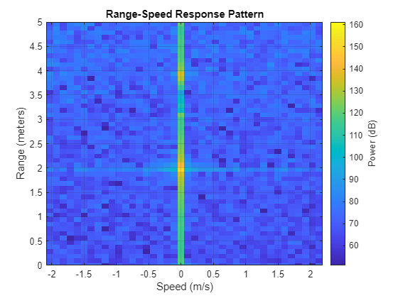
Although we can see the target near 2 meters with 0 velocity because we are using a corner reflector with a large radar cross section (RCS), it is somewhat difficult in this 2D image because there is stationary clutter present in the indoor environment where the data was collected.

To further investigate, we can visualize just the range and Doppler slice where the reflector is present. To do so, we calculate the range-Doppler response, and then determine the range and Doppler index of the reflector by searching the visible area for the maximum magnitude signal.

% Calculate the range-Doppler response
[resp,range,speed] = rdResponse(stationaryReflectorData);

% Get the response in the search area
visibleRangeIdx = range >= minDisplayRange & range <= maxDisplayRange;
visibleRange = range(visibleRangeIdx);
visibleResp = resp(visibleRangeIdx,:,:);

% Extract the first antenna element response in the image
firstElementResponse = squeeze(visibleResp(:,1,:));

% Determine the location of the maximum response
[~,tgtIdx] = max(abs(firstElementResponse(:)));
[stationaryTgtRangeIdx,stationaryTgtDopIdx] = ind2sub(size(firstElementResponse),tgtIdx);

With the reflector location measured, we can plot the range and Doppler response for each of the virtual antenna elements at just the slice where the reflector is located using helperPlotRangeDopplerSlice.

helperPlotRangeDopplerSlice(visibleResp,visibleRange,speed,stationaryTgtRangeIdx,stationaryTgtDopIdx);

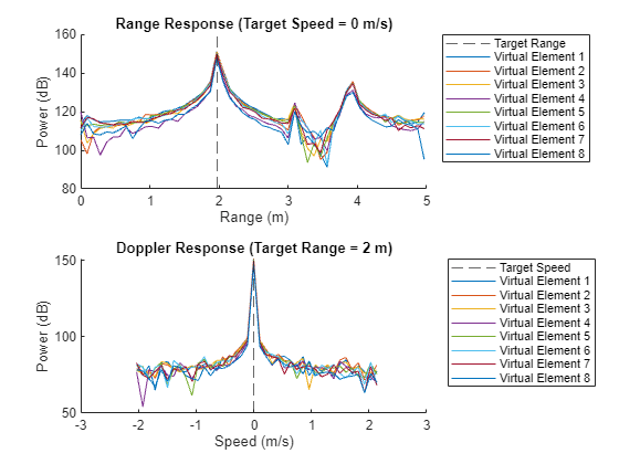
We can clearly see the reflector response in the range and Doppler slices. Furthermore, we see that the response for each of the antenna elements is very similar. In the range response we also see some lower power peaks at ranges further than our target. This is expected, because we are seeing the range response at 0 Doppler, meaning all of the stationary clutter surrounding the target will be visible.

Single Moving Reflector

We go through the same visualizations in this section, but the data cube was collected with someone walking slowly (~1 mph) in front of the radar holding the corner reflector. Once again, we load a data snapshot and arrange it into a virtual array.

load(dataFilePath,'movingReflectorData');
movingReflectorData = helperArrangeVirtualData(movingReflectorData,radarConfiguration);

We again plot the range-Doppler image for the first antenna element.

figure;
plotResponse(rdResponse,squeeze(movingReflectorData(:,1,:)));
ylim([minDisplayRange maxDisplayRange]);

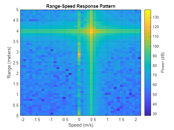
In this case, it is easier to see the reflector response. This is because the reflector is now moving, so it is not being obscured by stationary clutter in Doppler space. The reflector appears to be moving at ~0.5 m/s (~1 mph), which aligns with the slow walking speed that was used to collect data.

Note that although the reflector is moving towards the radar and thus has a negative range rate, it's speed on the figure is shown to be positive. This is because the speed as defined by phased.RangeDopplerResponse is the radialspeed, which has the opposite sign as the range rate. This will be important when we generate detections, because we will flip the sign of the relative radial speed to be consistent with range rate.

In order to look at the range and Doppler slices where the targets are located, we once again calculate the range-Doppler response and then determine the range and Doppler index of the reflector.

% Calculate the range-Doppler response
[resp,range,speed] = rdResponse(movingReflectorData);

% Get the response in the search area
visibleRangeIdx = range >= minDisplayRange & range <= maxDisplayRange;
visibleRange = range(visibleRangeIdx);
visibleResp = resp(visibleRangeIdx,:,:);

% Extract the first antenna element response in the image
firstElementResponse = squeeze(visibleResp(:,1,:));

% Determine the location of the maximum response
[~,tgtIdx] = max(abs(firstElementResponse(:)));
[stationaryTgtRangeIdx,stationaryTgtDopIdx] = ind2sub(size(firstElementResponse),tgtIdx);

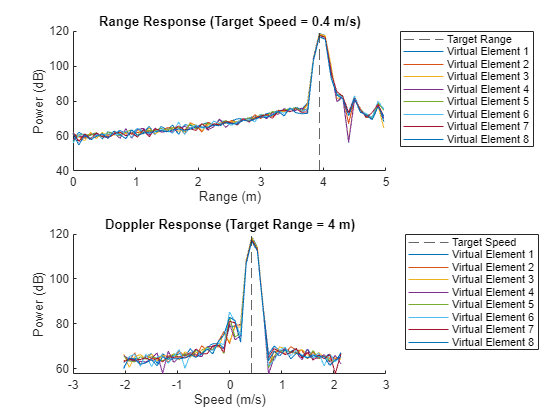
With the reflector location measured, we can plot the range and Doppler response for each of the virtual antenna elements at just the slice where the reflector is located using helperPlotRangeDopplerSlice.

helperPlotRangeDopplerSlice(visibleResp,visibleRange,speed,stationaryTgtRangeIdx,stationaryTgtDopIdx); 

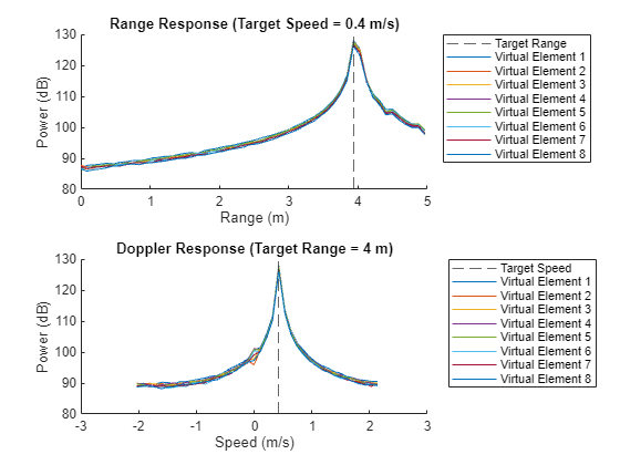
With the moving reflector, it is easier to see the response in range and Doppler space because of the lack of interfering clutter. In the next section, we look at using a windowing function to reduce the sidelobe level of the range and Doppler response.

Windowing Function

Oftentimes a windowing function is used to reduce the range and Doppler sidelobes in the measured response, making it easier to detect and resolve nearby targets. Although windowing can reduce sidelobes, it doesn't come without a cost. Using a windowing function will widen the peak and reduce the maximum power of the response.

In this section we choose to look only at the moving reflector data because this avoids interference from static clutter, which makes it easier to see the effect of the windowing function.

In order to investigate the impact of a windowing function on the range and Doppler response sidelobes, we create a new phased.RangeDopplerResponse object that utilizes Hamming windowing functions.

rdResponseWindowed = phased.RangeDopplerResponse(RangeMethod="FFT",...
    DechirpInput=false,SampleRate=fs,SweepSlope=sweepSlope,...
    DopplerOutput='Speed',OperatingFrequency=fc,PRFSource='Property',...
    PRF=prf,RangeWindow='Hamming',DopplerWindow='Hamming');

We can once again plot the range-Doppler image for the first antenna to see how the response is affected by windowing.

figure;
plotResponse(rdResponseWindowed,squeeze(movingReflectorData(:,1,:)));
ylim([minDisplayRange maxDisplayRange]);

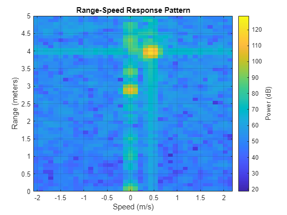
Comparing this image to the image when no windowing function was used, we can see that the target response widens in both range and Doppler, but the spread across range and Doppler space also appears to be reduced significantly.

We can also look at just the range and Doppler slices where the reflector is located for the moving reflector data for additional clarity.

% Calculate the range-Doppler response
respWindow = rdResponseWindowed(movingReflectorData);

% Get the response in the search area
visibleRespWindow = respWindow(visibleRangeIdx,:,:);

% Plot the responses at the target index
helperPlotRangeDopplerSlice(visibleRespWindow,visibleRange,speed,stationaryTgtRangeIdx,stationaryTgtDopIdx); 

In comparing the responses that were calculated using windowing functions to the original responses for the moving reflector, there are a few important points to consider. We can see that in the windowed responses, the peak of the response decreased ~10 dB from 130 to 120 dB and the width of the responses both increased. However, in both cases, the sidelobe levels reduced substantially meaning that the peak-to-sidelobe ratio is increased.

Depending on the goal of the signal processing routine, you may or may not want to use a windowing function to reduce the sidelobes. If location accuracy is the most important consideration, then the widening of the main response due to the windowing functions is undesirable. For the purposes of this example, we are most interested in ensuring that we detect targets that are present, so in our detection generation algorithm we calculate the range-Doppler response using a windowing function.

Range-Doppler Coupling

Another consideration when calculating the range response of an FMCW waveform is that the dechirp frequency is a function of both range and range-rate of the target. This phenomenon is known as range-Doppler coupling. This coupling could introduce errors in our range analysis if we ignore the effect. To determine if we need to consider this effect, we calculate the expected range error introduced by the fastest moving target that we will be observing. We assume that the fastest moving target that we will observe is a person walking briskly at 4 mph (1.8 m/s).

fastTarget = 1.8;
fd = 2*speed2dop(fastTarget,lambda);
rangeOffset = rdcoupling(fd,sweepSlope)

rangeOffset = 
-0.0055

The range offset introduced by Doppler coupling in the worst case is low enough that we will ignore it for the sake of this example, however it may be important to consider depending on the application.

Angle Response

In addition to range and speed, we are interested in determining the angular location, or bearing of the target with respect to the radar. Because we have a one-dimensional virtual array, we can resolve the direction of the target in one dimension. For this example, we orient the radar so that the array axis is parallel to the ground in order to resolve the target azimuth. However, the radar could also be oriented such that the array axis is perpendicular to the ground, allowing the target elevation to be resolved.

In this example, we work under the assumption that the target is present in the far field, meaning that we assume radar returns arriving at the array are planar. The Fraunhofer distance is typically used as the transition distance between the near and far field of an antenna, and is defined as:

$$\mathit{d}=\frac{2{\mathit{D}}^2}{\lambda }$$

Where $\mathit{D}$ is the largest dimension of the radiator and $\lambda$ is the wavelength. We can compute the Fraunhofer distance for the virtual array:

elempos = getElementPosition(virtualArray);
minpos = min(elempos,[],2);
maxpos = max(elempos,[],2);
D = max(maxpos-minpos);
dfraunhofer = (2*D^2)/lambda;
disp(['Far field starts at ',num2str(dfraunhofer),' m']);

Far field starts at 0.095389 m

Therefore, it is safe to assume that our targets of interest will be in the far field in this example.

The data used in this section is a snapshot that was collected with a corner reflector target placed with an azimuth of 20 degrees.

load(dataFilePath,'angleTargetData');
angleTargetData = helperArrangeVirtualData(angleTargetData,radarConfiguration);

We are interested in verifying that the angle response of each alternating transmit-receive group as well as the angle response of the whole virtual array matches our expectations. First, we look at a single transmit-receive group.

Single Transmit-Receive Group Angle Response

As discussed in a previous section, we form a virtual array by alternating transmissions between transmit antennas. Before looking at the angle response of the entire virtual array, we analyze the angle response for a single transmit-receive group to verify that it matches our expectations. To do so, we create a phased.RangeAngleResponse object using just the receive array as the sensor.

% Single transmit-receive group RangeAngleResponse
receiveRaResponse = phased.RangeAngleResponse(RangeMethod="FFT",...
    DechirpInput=false,SampleRate=fs,SweepSlope=sweepSlope,...
    SensorArray=rxArray,OperatingFrequency=fc);

Data is extracted for the first chirp in the range that we wish to display for just the first group of receive antennas.

% Get the first chirp for just the first group of recieve antennas
rxGroup = find(radarConfiguration.ActiveReceivers);
angleTargetFirstChirp = angleTargetData(:,rxGroup,1);

A reflector was placed at approximately twenty degrees, so we would expect that the angle response would be maximized at this angle at the target range. We plot the range-angle response below using the plotResponse method to test this assumption for the first transmit-receive group.

figure;
plotResponse(receiveRaResponse,angleTargetFirstChirp);
ylim([minDisplayRange maxDisplayRange]);

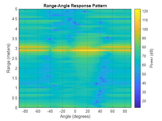
As we did with the range-Doppler response, we can look at the range-angle response for just the range slice where the target is present to get a better sense of the response characteristics than is visible in the 2-D range-angle response. We can also compare the response to the response that we expect given the geometry of the receive array.

To do so, we first calculate the range-angle response and estimate the reflector location by getting the range and angle of the maximum response value in the visible region shown above.

% Get the target range and angle index
[resp,range,ang] = receiveRaResponse(angleTargetFirstChirp);

% Get the response in the search area
visibleRangeIdx = range >= minDisplayRange & range <= maxDisplayRange;
visibleRange = range(visibleRangeIdx);
visibleResp = resp(visibleRangeIdx,:,:);

% Determine the location of the maximum response
[~,tgtIdx] = max(abs(visibleResp(:)));
[angleTgtRangeIdx,angleTgtAngleIdx] = ind2sub(size(visibleResp),tgtIdx);

% Get the range and angle of the target
targetRange = visibleRange(angleTgtRangeIdx);
targetAzimuth = ang(angleTgtAngleIdx);

% Get the angle response at the target range
measuredResponse = visibleResp(angleTgtRangeIdx,:);

Next, we calculate the expected angle response given the measured target angle. We first simulate a signal arriving at our receive array using the collectPlaneWave method on the array model. We use a signal value of 1 because we are interested in generating an expected response. We then calculate a steering vector at each response angle of interest based on the antenna geometry and apply the steering vectors to the received signal.

% Simulate a signal arriving in the direction of the reflector
targetAngle = [targetAzimuth;0];
simRxSig = collectPlaneWave(rxArray,1,targetAngle,fc);

% Apply steering weights to the received signal to get response
nSteerAngles = numel(ang);
steerAngles = [ang';zeros(1,nSteerAngles)];
steerWeights = steervec(getElementPosition(rxArray)/lambda,steerAngles);
expectedResponse = simRxSig*conj(steerWeights);

Using the following helper function we plot the actual and expected angle response due to the position of the reflector.

helperPlotSingleAngleResponse(ang,measuredResponse,targetRange,targetAzimuth,expectedResponse);

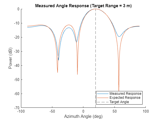
We can see that the measured response and the expected response generally agree. The main beam has a similar width, the sidelobe nulls are in the same locations, and the sidelobe levels are similar.

There are many real-world factors that the expected response doesn't account for which are each at least partially response for explaining the differences between the measured and expected angle response. To list a few, the expected response does not model:

1. The individual pattern of each antenna element

2. Hardware impairments

3. Multipath

4. Clutter

5. Calibration errors

6. Positional placement errors in the antenna locations

Even ignoring these important effects, the measured response is close enough to the expected response to instill confidence that the radar and processing algorithms are working as expected.

Virtual Array Angle Response

Now that we have confirmed that the angle response matches our expectation for a single transmit-receive group, we turn our attention to the response of the entire virtual array. We once again create a phased.RangeAngleResponse, but now the sensor is the virtual array instead of a single receive array. The virtual array contains 2x as many antenna elements as a single receive array, so we would expect the main beam to be much narrower.

% Single transmit-receive group RangeAngleResponse
virtualRaResponse = phased.RangeAngleResponse(RangeMethod="FFT",...
    DechirpInput=false,SampleRate=fs,SweepSlope=sweepSlope,...
    SensorArray=virtualArray,OperatingFrequency=fc);

We view the range-angle response for the first chirp for the entire virtual array. We use the same set of data with a reflector placed at approximately 20 degrees azimuth.

figure;
angleTargetFirstChirp = angleTargetData(:,:,1);
plotResponse(virtualRaResponse,angleTargetFirstChirp);
ylim([minDisplayRange maxDisplayRange]);

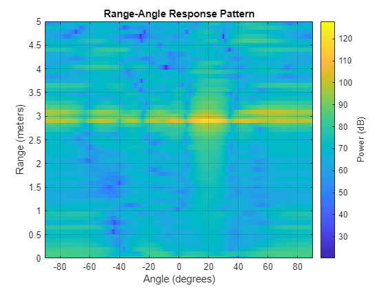
Using the virtual array, we can see that the angle response is narrower than for a single transmit-receive pair. This confirms that by using the virtual array technique, we can substantially improve the azimuth resolution of the radar.

We again look at a single range cut for the virtual array angle response and compare it to the expected response. We use the same target location that was calculated in the previous section, and use the same approach to generate an expected response.

% Calculate the range-angle response for the virtual array
[resp,range,ang] = virtualRaResponse(angleTargetFirstChirp);

% Get the response in the visible area
visibleResp = resp(visibleRangeIdx,:,:);

% Get the angle response at the target range
measuredResponse = visibleResp(angleTgtRangeIdx,:);

% Simulate a signal arriving in the direction of the reflector
simRxSig = collectPlaneWave(virtualArray,1,targetAngle,fc);

% Apply steering weights to the received signal to get response
nSteerAngles = numel(ang);
steerAngles = [ang';zeros(1,nSteerAngles)];
steerWeights = steervec(getElementPosition(virtualArray)/lambda,steerAngles);
expectedResponse = simRxSig*conj(steerWeights);

% Plot the measured response vs. the expected response
helperPlotSingleAngleResponse(ang,measuredResponse,targetRange,targetAzimuth,expectedResponse);

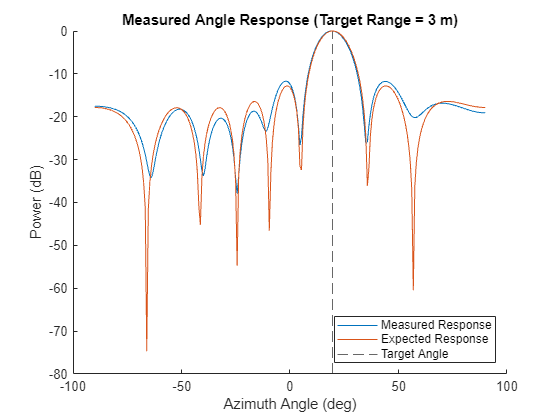
The measured angle response for the virtual array also closely matches the calculated response.

Detection Generation

Now that we have sufficiently familiarized ourselves with the radar being used to capture data, we develop a pipeline that generates detections with range, range rate, and azimuth information. The detection generation pipeline is summarized by the following schematic:

There are an infinite number of ways to generate detections from radar I/Q data. The process outlined here is one example, but any of the steps above could be altered, reordered, removed, or combined with other steps depending on the application, available hardware, and system requirements.

Before running the detection generation scenario, we discuss each step of the detector below.

Rearrange Virtual Array Data

The purpose of this step is to arrange the output data cube into the virtual array format. This step was discussed in Antenna Geometry. To rearrange the data, we use the helperArrangeVirtualData function.

Moving Target Indicator (MTI) Filter

We expect that there will be substantial static clutter visible as we can see in the Range-Doppler Response section. Because the goal is to detect people, we would like to ignore this static clutter. There are many approaches for ignoring static clutter returns from radar data. Once such approach is an MTI filter which removes these returns from the signal altogether by applying a high pass filter across the slow-time dimension. The MTI filter that we use in this example is a finite impulse response (FIR) filter with the following coefficients:

mtiCoeff = [1 -2 1];

One important point to note is that FIR filters have a transient period during which there may be some unexpected behavior. This transient period lasts as long as the number of non-zero delay coefficients. For the MTI filter described above, the transient period lasts for a total of 2 pulses. This will need to be accounted for during processing. We will do so by applying the MTI filter and then ignoring the pulses in the transient period.

numPulseTransient = numel(mtiCoeff)-1;

For more information on MTI filters, see Ground Clutter Mitigation with Moving Target Indication (MTI) Radar.

Range-Doppler Processing

The purpose of this step is to estimate the range and speed of the target as well as achieve some coherent processing gain. As discussed in the Range-Doppler Response section, we use windowing functions in order to reduce sidelobes.

preprocessRangeDopplerResponse = phased.RangeDopplerResponse(RangeMethod="FFT",...
    DechirpInput=false,SampleRate=fs,SweepSlope=sweepSlope,...
    DopplerOutput='Speed',OperatingFrequency=fc,PRFSource='Property',...
    PRF=prf,RangeWindow='Hamming',DopplerWindow='Hamming');

Beamforming

After range-Doppler processing, we want to beamform to a small number of azimuth angles. The purpose of this step is to take advantage of spatial processing gain prior to generating detections, and to get an initial estimate of the target azimuth. To do so, we use the phased.PhaseShiftBeamformer, which uses the same underlying approach that is used by the phased.RangeAngleResponse.

In order to determine the angles that we would like to beamform towards, we look at the response pattern of the virtual array. We use the simulated antenna pattern for the analysis in this section having already established the similarity between the measured and expected angle response of the virtual array in Virtual Array Angle Response section.

ax = axes(figure);
patternAngles = -90:90;
pattern(virtualArray,fc,patternAngles,0,CoordinateSystem='rectangular',Parent=ax);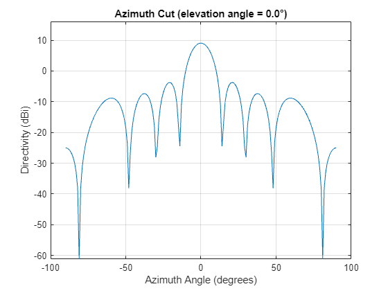

arrayPattern = pattern(virtualArray,fc,patternAngles,0,CoordinateSystem='rectangular',Parent=ax);

We wish to beamform to the smallest number of angles that will allow us to cover our field of view (FOV) while allowing some tolerable amount of scalloping loss between beams.

For this example, we use 9 dB as the acceptable loss between beams, although this can be adjusted based on the power requirements.

To determine our beamforming angles, we first determine the 9 dB beamwidth based on the simulated pattern.

patternMax = max(arrayPattern);
allowedLoss = 9;
mainLobeAngles = patternAngles(arrayPattern >= (patternMax - allowedLoss));
beamwidth = mainLobeAngles(end)-mainLobeAngles(1);

We then select our beamforming angles so that the main lobes of our beams cover the desired FOV. For this example, we establish the FOV as -30 to 30 degrees.

fovStart = -30;
fovStop = 30;
beamformingAngles = fovStart+beamwidth/2:beamwidth/2:fovStop-beamwidth/2;

The response of the virtual array steered to these beamforming angles shows that these angles will give us good coverage of the FOV.

ax = axes(figure);
hold(ax,"on")
for iAng = 1:length(beamformingAngles)
    sv = steervec(getElementPosition(virtualArray)/lambda,beamformingAngles(iAng));
    pattern(virtualArray,fc,-90:90,0,CoordinateSystem='rectangular',Weights=sv,Parent=ax);
end
legend(ax,"hide");

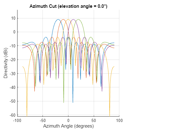
We create our beamformer with the calculated beamforming angles.

preprocessBeamformer = phased.PhaseShiftBeamformer(SensorArray=virtualArray,...
    OperatingFrequency=fc,Direction=[beamformingAngles;zeros(1,numel(beamformingAngles))]);

2D Constant False Alarm Rate (CFAR) Detector

For initial detection generation, we use a 2D CFAR detector. This detector will operate on each beamformed range-Doppler image. We use 5 guard cells in the range dimension and 1 guard cell in the Doppler dimension to avoid the sidelobes based on the plots in the Range-Doppler Response section. We use 10 training cells in the range dimensions and 2 training cells in the Doppler dimension.

rangeGuard = 5;
dopplerGuard = 1;
rangeTrain = 10;
dopplerTrain = 2;
pfa = 1e-6;
cfar = phased.CFARDetector2D(GuardBandSize=[rangeGuard dopplerGuard],...
    TrainingBandSize=[rangeTrain dopplerTrain],ProbabilityFalseAlarm=pfa);

We only generate detections at ranges greater than 1 meter less than 15 meter, and with a speed greater than 0.2 m/s. Also, we do not test cells with guard or training cells outside of the acceptable region. We set up cell-under-test indices below based on these requirements.

% Set min and max cell-under-test range and speed
minRange = 1;
maxRange = 15;
minSpeed = 0.2;
maxSpeed = Inf;

% Set min and max acceptable cell-under-test index based on guard and
% training cells
minRangeCell = rangeGuard + rangeTrain + 1;
minDopplerCell = dopplerTrain + dopplerGuard + 1;
maxRangeCell = length(range) - minRangeCell + 1;
maxDopplerCell = length(speed) - minDopplerCell + 1 - numPulseTransient;

% Update speed to have the correct number of samples for transient pulse
% removal due to MTI filter
speed = linspace(speed(1),speed(end),numel(speed)-numPulseTransient)';

% Get range and doppler indices
rangeIdx = (1:length(range))';
dopplerIdx = (1:length(speed))';

% Get cell-under-test indices for range and Doppler
rangeCutIdx = find(range >= minRange & range <= maxRange & rangeIdx >= minRangeCell & rangeIdx <= maxRangeCell);
dopplerCutIdx = find(abs(speed) >= minSpeed & abs(speed) <= maxSpeed & dopplerIdx >= minDopplerCell & dopplerIdx <= maxDopplerCell);

% Generate cell-under-test pairs
[p,q] = meshgrid(rangeCutIdx, dopplerCutIdx);
cutidx = [p(:)';q(:)'];

The area in the following image shows the range-Doppler region that will be tested by our 2D CFAR detector.

helperDrawCellsUnderTest(range,speed,cutidx);

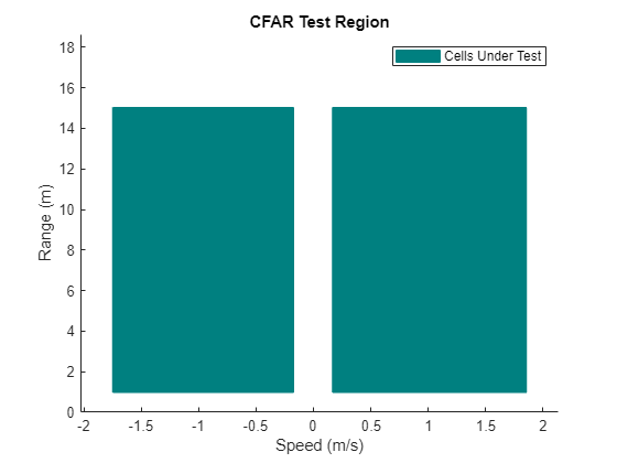
The Cells Under Test region labelled in the figure above contains all of the cells that will be tested for the presence of detections by the CFAR detector.

Direction of Arrival (DOA) Estimation

After generating detections with the 2D CFAR detector, we assign each detection a direction of arrival estimate.

We will only perform the DOA estimation around the beamforming angle that gave the maximum range-Doppler response instead of scanning the entire FOV. We do this for the sake of efficiency. If the beamforming angle that gave the maximum response is the first or last beamforming angle, then our DOA scan region will go out to +- 90 degrees. We use a 1-degree DOA scan resolution.

doaScanAngles = [-90 beamformingAngles 90];
doaScanRes = 1;

We use the phased.BeamscanEstimator2D and make the assumption that there is only a single target located in the given range-Doppler bin.

doaEstimator = phased.BeamscanEstimator2D(SensorArray=virtualArray,...
    OperatingFrequency=fc,ElevationScanAngles=0,...
    DOAOutputPort=true);

People Detection Demonstration

We can configure the final part of this example for data playback or for data streaming. To run this example yourself, connect a TI mmWave IWR1642BOOST radar sensor and set the control to "Streaming".

runMode = "Playback";

% Create a helper class to run this section depending on whether streaming
% or playback is selected
switch runMode
    case "Playback"
        detectionProcessHelper = helperPlaybackDetectionProcess(dataFilePath,videoFilePath);
    case "Streaming"
        nRuns = 500;
        detectionProcessHelper = helperStreamingDetectionProcess(model,nRuns);
end

We create a range-angle scope and a range-Doppler scope to visualize the collected data.

% Create scopes
rascope = phased.RangeAngleScope(IQDataInput=false);
rdscope = phased.RangeDopplerScope(IQDataInput=false,DopplerLabel="Speed (m/s)");

% Open scopes with all zero data
startRange = 0;
endRange = 10;
showRangeIdx = range >= startRange & range <= endRange;
showRange = range(showRangeIdx);
angles = linspace(virtualRaResponse.AngleSpan(1),virtualRaResponse.AngleSpan(2),virtualRaResponse.NumAngleSamples)';
initRaData = zeros(numel(showRange),numel(angles));
initRdData = zeros(numel(showRange),numel(speed));
rascope(initRaData,showRange,angles);
rdscope(initRdData,showRange,speed);

In addition to these scopes, we create a display to show detections alongside video data of the capture scene. The display used for this section is adapted from People Tracking Using TI mmWave Radar (Sensor Fusion and Tracking Toolbox). This display allows us to show the detections alongside images to make it easier to understand whether the radar is generating detections where we expect. We only show images in playback mode. In streaming mode, we just show the location of detections.

display = getDisplay(detectionProcessHelper);

The output of our detection algorithm are objectDetection objects. For each detection, we provide range, range rate, and azimuth angle. The measurement noise for the detection comes from the azimuth resolution, range resolution, and range rate resolution of the system.

rangeResolution = radarConfiguration.RangeResolution;
azimuthResolution = radarConfiguration.AzimuthResolution;
speedResolution = radarConfiguration.RangeRateResolution;
measurementParameters = struct(Frame='spherical',HasElevation=false);
measurementNoise = eye(3).*[rangeResolution;azimuthResolution;speedResolution];

Finally, we loop through the collected data or stream live data and generate detections.

while runAnotherLoop(detectionProcessHelper)
    
    % collect data
    [radarData,imageData,time] = captureData(detectionProcessHelper);

    % Step 1: Rearrange Virtual Array Data

    virtualData = helperArrangeVirtualData(radarData,radarConfiguration);

    % Step 2: MTI Filter
    
    % Apply filter and remove pulses in transient region
    virtualData = filter(mtiCoeff,1,virtualData,[],3);
    virtualData = virtualData(:,:,numPulseTransient+1:end);

    % Step 3: Range-Doppler Processing

    [rdProcess,range,speed] = preprocessRangeDopplerResponse(virtualData);
    showRangeIdx = range >= startRange & range <= endRange;

    % Step 4: Beamforming

    % Beamform each range-Doppler slice
    nSample = size(rdProcess,1);
    nAngs = size(preprocessBeamformer.Direction,2);
    nDoppler = size(rdProcess,3);
    bfData = zeros(nSample,nAngs,nDoppler);
    for iDoppler = 1:nDoppler
        bfData(:,:,iDoppler) = preprocessBeamformer(rdProcess(:,:,iDoppler));
    end

    % Step 5: 2D CFAR

    bfData = permute(bfData,[1 3 2]);
    allDetIdx = cfar(abs(bfData).^2,cutidx);
    detIdx = find(sum(allDetIdx,2) > 0);

    % Step 6: Get DOA for each detection

    % Create a new detection object for each detection
    nDetection = numel(detIdx);
    detections = cell(1,nDetection);
    for iDet = 1:nDetection

        % Get range and Doppler detection indices
        cIdx = detIdx(iDet);
        rangeIdx = cutidx(1,cIdx);
        cRange = range(rangeIdx);
        dopIdx = cutidx(2,cIdx);
        cSpeed = speed(dopIdx);

        % Get the max beamform response, determine DOA scan region
        [~,bfIdx] = max(abs(squeeze(bfData(rangeIdx,dopIdx,:))));
        doaScanStart = doaScanAngles(bfIdx);
        doaScanStop = doaScanAngles(bfIdx+2);
        scanAngles = doaScanStart:doaScanRes:doaScanStop;
        
        % Setup DOA estimator
        if ~isequal(doaEstimator.AzimuthScanAngles,scanAngles)
            release(doaEstimator);
            doaEstimator.AzimuthScanAngles = scanAngles;
        end

        % Get DOA estimate
        rdSlice = rdProcess(rangeIdx,:,dopIdx);
        [est,cDoa] = doaEstimator(rdSlice);
        detections{iDet} = objectDetection(time,[cDoa(1);cRange;-cSpeed],MeasurementParameters=measurementParameters,MeasurementNoise=measurementNoise);
    end

    % Visualize detections

    % Display detections
    display(detections, {}, {}, imageData);

    % Display range-Doppler response beamformed to boresight
    bfBoresightRd = bfData(:,:,beamformingAngles == 0);
    rdscope(abs(bfBoresightRd(showRangeIdx,:)).^2,range(showRangeIdx),speed);

    % Display range-angle response for middle
    [raresp,range,angle] = virtualRaResponse(virtualData(:,:,1));
    rascope(abs(raresp(showRangeIdx,:)).^2,range(showRangeIdx),angle);
end

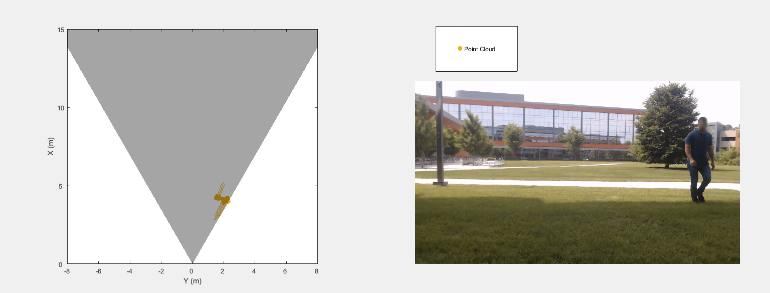
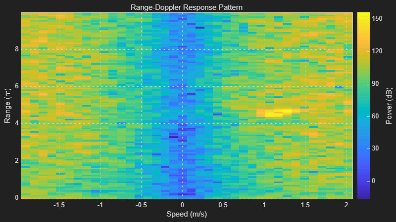
By combining a detection generation algorithm such as the one shown in this example with a tracker such as the one used in People Tracking Using TI mmWave Radar (Sensor Fusion and Tracking Toolbox), we could create a full end-to-end people tracking radar.

Conclusion

In this example we collect I/Q data from a TI mmWave radar and investigate the range, Doppler, and angle response properties of the radar. Based on this investigation, we develop a simple detection generation algorithm tuned for detection of people. This serves as an introduction to collecting and processing I/Q data in MATLAB® with the TI mmWave radar.

Helper Functions

Plot the range and Doppler response of each virtual element at the specified indices.

function helperPlotRangeDopplerSlice(rdresp,range,speed,tgtrangeidx,tgtdopidx)
    f = figure;
    tiledlayout(f,'vertical');
    
    % Get target range and speed
    tgtRange = range(tgtrangeidx);
    tgtSpeed = speed(tgtdopidx);

    % Setup range axes
    rangeRespAx = nexttile;
    hold(rangeRespAx,"on");
    title(rangeRespAx,['Range Response (Target Speed = ',num2str(tgtSpeed,1),' m/s)']);
    xlabel(rangeRespAx,'Range (m)');
    ylabel(rangeRespAx,'Power (dB)');
    xline(rangeRespAx,tgtRange,DisplayName='Target Range',LineStyle='--');

    % Setup Doppler axes
    dopRespAx = nexttile;
    hold(dopRespAx,"on");
    title(dopRespAx,['Doppler Response (Target Range = ',num2str(tgtRange,1),' m)']);
    xlabel(dopRespAx,'Speed (m/s)');
    ylabel(dopRespAx,'Power (dB)');
    xline(dopRespAx,tgtSpeed,DisplayName='Target Speed',LineStyle='--');

    nAntenna = size(rdresp,2);
    for iAntenna = 1:nAntenna
        name = ['Virtual Element ',num2str(iAntenna)];
        
        % plot range slice
        rangeSlice = squeeze(rdresp(:,iAntenna,tgtdopidx));
        plot(rangeRespAx,range,mag2db(abs(rangeSlice)),DisplayName=name);

        % Plot Doppler slice
        dopSlice = squeeze(rdresp(tgtrangeidx,iAntenna,:));
        plot(dopRespAx,speed,mag2db(abs(dopSlice)),DisplayName=name);
    end

    legend(rangeRespAx,"show",Location="northeastoutside");
    legend(dopRespAx,"show",Location="northeastoutside");
end

Plot the angle response for a single range and chirp.

function helperPlotSingleAngleResponse(az,targetAngResp,targetRange,targetAngle,calculatedResponse)
    % Plot measured and calculated response
    ax = axes(figure);
    hold(ax,"on");
    xlabel(ax,'Azimuth Angle (deg)');
    ylabel(ax,'Power (dB)');
    measuredRespNorm = mag2db(abs(targetAngResp)./max(abs(targetAngResp)));
    calculatedRespNorm = mag2db(abs(calculatedResponse)./max(abs(calculatedResponse)));
    plot(ax,az,measuredRespNorm,DisplayName='Measured Response');
    plot(ax,az,calculatedRespNorm,DisplayName='Expected Response');
    xline(ax,targetAngle,DisplayName="Target Angle",LineStyle="--");
    title(ax,['Measured Angle Response (Target Range = ',num2str(targetRange,1),' m)']);
    legend(ax,Location="southeast");
end

Draw the range-Doppler region under test.

function helperDrawCellsUnderTest(range,speed,cutidx)
    % Draw cells under test
    ax = axes(figure);
    hold(ax,"on");
    rangeWidth = abs(range(2)-range(1));
    speedWidth = abs(speed(2)-speed(1));
    for iIdx = 1:size(cutidx,2)
        rIdx = cutidx(1,iIdx);
        r = range(rIdx);
        rStart = r-rangeWidth/2;
        rStop = r+rangeWidth/2;
        sIdx = cutidx(2,iIdx);
        s = speed(sIdx);
        sStart = s-speedWidth/2;
        sStop = s+speedWidth/2;
        x = [sStart sStop sStop sStart];
        y = [rStart rStart rStop rStop];
        c = [0 0.5 0.5];
        p = patch(ax,x,y,c,EdgeColor=c);
    end
    set(ax,'YDir','normal');
    xlim(ax,[min(speed) max(speed)]);
    ylim(ax,[0 max(range)]);
    xlabel(ax,'Speed (m/s)');
    ylabel(ax,'Range (m)');
    title(ax,'CFAR Test Region');
    p.DisplayName = 'Cells Under Test';
    legend(p);
end