Train Reinforcement Learning Agent Offline to Control Quanser QUBE Pendulum

This example shows how you can train an agent from existing data instead of using an environment. Training an agent from data (offline reinforcement learning) can be useful to efficiently prototype different design choices by leveraging already collected data. In this example, two reinforcement learning (RL) agents are trained to swing up and balance a Quanser QUBE™-Servo 2 inverted pendulum system. First, you train a TD3 agent online using a Simulink® environment and collect training data using a data logger. Then, you train another TD3 agent offline using the collected data and a modified reward function to achieve a different behavior from the agent. You then compare the behavior of both agents.

Inverted Pendulum Model

The Quanser QUBE-Servo 2 pendulum system is a rotational inverted pendulum with two degrees of freedom. It is non-linear, underactuated, non-minimum phase, and it is modeled in Simulink using Simscape™ Electrical™ and Simscape Multibody™. For a detailed description of the dynamics, see [1]. For related examples that use this pendulum system model, see Train Reinforcement Learning Agents to Control Quanser QUBE Pendulum and Run SIL and PIL Verification for Reinforcement Learning.

The pendulum is attached to the motor arm through a free revolute joint. The arm is actuated by a DC motor. The environment has the following properties:

• The angles and angular velocities of the motor arm ($\theta$,$\dot{\theta }$) and pendulum ($\varphi$,$\dot{\varphi }$) are measurable.

• The motor is constrained to $|\theta |\le 5\frac{\pi }{8}\mathrm{rad}$ and $|\dot{\theta }|\le 30\frac{\mathrm{rad}}{\sec }$.

• The pendulum is upright when $\varphi =0$.

• The motor input is constrained to $\pm 12\mathit{V}$.

• The agent action $\left(|\mathit{u}|\le 1\right)$ is scaled to the motor voltage in the environment.

Open the Simulink model.

mdl = "rlQubeServoModel";
open_system(mdl)

Define the angular and voltage limits, as well as the model's sample time.

theta_limit = 5*pi/8;
dtheta_limit = 30;
volt_limit = 12;
Ts = 0.005;

Train TD3 Agent Online

A TD3 agent is trained online against the Simulink enviroment. For this agent:

• The environment is the pendulum system modeled in Simscape Multibody.

• The observation is the vector ${\mathit{s}}_{\mathit{k}}=\left[\sin {\theta }_{\mathit{k}},\cos {\theta }_{\mathit{k}},\dot{{\theta }_{\mathit{k}}},\sin {\phi }_{\mathit{k}},\cos {\phi }_{\mathit{k}},\dot{{\phi }_{\mathit{k}}},{\mathit{u}}_{\mathit{k}-1}\right]$. Using the sine and cosine of the measured angles can facilitate training by representing the otherwise discontinuous angular measurements by a continuous two-dimensional parametrization.

• The action is the normalized input voltage command to the servo motor.

• The reward signal is defined as follows:

$$\begin{array}{l}\mathit{r}\left({\mathit{s}}_{\mathit{k}},{\mathit{u}}_{\mathit{k}-1}\right)={\mathit{F}}_{\mathit{k}}-0.1\left({{\theta }_{\mathit{k}}}^2+{\phi }_{\mathit{k}}^2+{\dot{{\theta }_{\mathit{k}}}}^2+{\dot{\phi }}^2+{\mathit{u}}_{\mathit{k}-1}^2+0.3{\left({\mathit{u}}_{\mathit{k}-1}-{\mathit{u}}_{\mathit{k}-2}\right)}^2\right)\\ {\mathit{F}}_{\mathit{k}}=\{\begin{array}{ll}1& {\theta }_{\mathit{k}}\in \pm 5\frac{\pi }{8}\mathrm{rad}\mathrm{and}\dot{{\theta }_{\mathit{k}}}\in \pm 30\frac{\mathrm{rad}}{\sec }\\ 0& \mathrm{otherwise}\end{array}\end{array}$$

The above reward function penalizes six different terms:

• Deviations from the forward position of the motor arm (${\theta }_{\mathit{k}}=0$)

• Deviations for the inverted position of the pendulum (${\phi }_{\mathit{k}}=0$)

• The angular speed of the motor arm $\dot{{\theta }_{\mathit{k}}}$

• The angular speed of the pendulum $\dot{{\varphi }_{\mathit{k}}}$

• The control action ${\mathit{u}}_{\mathit{k}}$

• Changes to the control action $\left({\mathit{u}}_{\mathit{k}-1}-{\mathit{u}}_{\mathit{k}-2}\right)$

The agent is rewarded while the system constraints are satisfied (that is ${\mathit{F}}_{\mathit{k}}=1$).

Set the random seed for reproducibility.

rng(0)

Create the input and output specifications for the agent. Set the action upper and lower limits to constrain the actions selected by the agent.

obsInfo = rlNumericSpec([7 1]);
actInfo = rlNumericSpec([1 1],UpperLimit=1,LowerLimit=-1);

Create the environment interface. Specify a reset function, defined at the end of the example, that sets random initial conditions.

agentBlk = mdl + "/RL Agent";
simEnv = rlSimulinkEnv(mdl,agentBlk,obsInfo,actInfo);
simEnv.ResetFcn = @localResetFcn;

To create an agent option object, use rlTD3AgentOptions. Specify sample time, experience buffer length, and the mini batch size.

agentOpts = rlTD3AgentOptions( SampleTime=Ts, ...
    ExperienceBufferLength=1e6, ...
    MiniBatchSize=128);
agentOpts.LearningFrequency = 1;
agentOpts.MaxMiniBatchPerEpoch = 1;

Specify the actor and critic optimizer options.

agentOpts.ActorOptimizerOptions.LearnRate = 1e-4;
agentOpts.ActorOptimizerOptions.GradientThreshold = 1;
agentOpts.CriticOptimizerOptions(1).LearnRate = 1e-3;
agentOpts.CriticOptimizerOptions(1).GradientThreshold = 1;
agentOpts.CriticOptimizerOptions(2).LearnRate = 1e-3;
agentOpts.CriticOptimizerOptions(2).GradientThreshold = 1;

Set to 64 the number of neurons in each hidden layer of the actor and critic networks. To create a default TD3 agent, use rlTD3Agent.

initOpts = rlAgentInitializationOptions(NumHiddenUnit=64);
TD3agent = rlTD3Agent(obsInfo,actInfo,initOpts,agentOpts);

Define training options. The length of an episode is given by the simulation time Tf divided by the sample time Ts.

Tf = 5;
maxSteps = ceil(Tf/Ts);

trainOpts = rlTrainingOptions(...
    MaxEpisodes=300, ...
    MaxStepsPerEpisode=maxSteps, ...
    ScoreAveragingWindowLength= 10, ...
    Verbose= false, ...
    Plots="training-progress",...
    StopTrainingCriteria="AverageReward",...
    StopTrainingValue=inf);

Create a data logger to save experiences that are later used for offline training of different agents. For more information, see rlDataLogger.

logger = rlDataLogger();
logger.EpisodeFinishedFcn = @localEpisodeFinishedFcn;
logger.LoggingOptions.LoggingDirectory = "SimulatedPendulumDataSet";

Train the TD3 agent using the Simulink environment using train. As shown in the following Reinforcement Learning Training Monitor screenshot, training can take over an hour, so you can save time while running this example by setting doTD3Training to false to load a pretrained agent. To train the agent yourself, set doTD3Training to true. During training, the experiences for each episode are saved in a file named loggedDataN.mat (where N is the episode number) in the SimulatedPendulumDataSet subfolder, under the current folder.

doTD3Training = false;
if doTD3Training
    trainStats = train(TD3agent,...
        simEnv,trainOpts,Logger=logger);    
else
    load("rlQuanserQubeAgents.mat","TD3agent");
end

Evaluate TD3 Agent

Test the trained agent and evaluate its performance. Since the environment reset function sets the intial state randomly, fix the seed of the random generator to ensure that the model uses the same initial conditions when running simulations.

testingSeed = 1;
rng(testingSeed)

For simulation, do not use an explorative policy.

TD3agent.UseExplorationPolicy = false;

Define simulation options.

numTestEpisodes = 1;
simOpts = rlSimulationOptions(...
    MaxSteps=maxSteps,...
    Numsimulations=numTestEpisodes);

Simulate the trained agent.

simResult = sim(TD3agent,simEnv,simOpts);

You can view the behavior of the trained agent in the mechanics explorer animation of the Simscape model, or you can plot a sample trajectory of the angles, control actions, and reward.

% Extract signals.
simInfo = simResult(1).SimulationInfo(1);
phi = get(simInfo.logsout,"phi_wrapped");
theta = get(simInfo.logsout,"theta_wrapped");
action = get(simInfo.logsout,"volt");
reward = get(simInfo.logsout,"reward");

% Plot values.
figure
tiledlayout(4,1)
nexttile
plot(phi.Values); title("Pendulum Angle")
nexttile
plot(theta.Values); title("Motor Arm Angle")
nexttile
plot(action.Values); title("Control Action")
nexttile
plot(reward.Values); title("Reward")

Train TD3 Agent Offline with a Modified Reward Function

Suppose you want to modify the reward function to encourage to balance the pendulum at a motor arm angle that matches some new reference angle$\beta$. Consider the new reward function:

$${\mathit{r}}^{\prime }\left({\mathit{s}}_{\mathit{k}},{\mathit{u}}_{\mathit{k}-1}\right)={\mathit{F}}_{\mathit{k}}-0.1\left({\left({\theta }_{\mathit{k}}-\beta \right)}^2+{\phi }_{\mathit{k}}^2+{\dot{{\theta }_{\mathit{k}}}}^2+{\dot{\phi }}^2+{\mathit{u}}_{\mathit{k}-1}^2+0.3{\left({\mathit{u}}_{\mathit{k}-1}-{\mathit{u}}_{\mathit{k}-2}\right)}^2\right)$$,

where $\beta$ corresponds to the desired angle that the motor arm should target. By expanding the modifed term, you can express the reward function in terms of the original reward.

$${\mathit{r}}^{\prime }\left({\mathit{s}}_{\mathit{k}},{\mathit{u}}_{\mathit{k}-1}\right)=\mathit{r}\left({\mathit{s}}_{\mathit{k}},{\mathit{u}}_{\mathit{k}-1}\right)-0.1\left(-2\beta {\theta }_{\mathit{k}}+\beta {}^2\right)$$

Instead of modifying the environment and training in simulation, you can leverage the already collected data to train the new agent offline. This process can be faster and more computationally efficient.

To train an agent from data you can:

1. Define a ReadFcn function that reads the collected files and returns data in appropriate form. If necessary, this function can also modify data (to change the reward, for example).

2. Create a fileDatastore object pointing to the collected data.

3. Create the agent to be trained.

4. Define training options.

5. Train the agent using trainFromData.

If, in the previous section, you have loaded the pre-trained TD3 agent instead of training the new agent, then at this point you do not have the training data in your local disk. In this case, download the data from the MathWorks® server, and unzip it to recreate the same folder and files that would exist after training the agent. If you already have the training data in the previously defined logging directory, set downloadData to false to avoid downloading the data.

downloadData = true;
if downloadData
    zipfilename = "SimulatedPendulumDataSet.zip";
    filename = ...
        matlab.internal.examples.downloadSupportFile("rl",zipfilename);
    unzip(filename)
end

Set the random seed for reproducibility.

rng(0)

Define the fileDatastore that points to the collected training data. Use the ReadFcn function of the data store to add the additional term to the reward of each experience. You can find the read function used in this example at the end of the example.

dataFolder = fullfile( ...
    logger.LoggingOptions.LoggingDirectory, ...
    "loggedData*.mat");
fds = fileDatastore(dataFolder, ...
    ReadFcn=@localReadFcn, ...
    FileExtensions=".mat");
fds.shuffle();

To create an agent option object, use rlTD3AgentOptions. Specify sample time, experience buffer length, and the mini batch size.

agentOpts = rlTD3AgentOptions( ...
    SampleTime=Ts,...
    ExperienceBufferLength=1e6,...
    MiniBatchSize=128);

Specify the actor and critic optimizer options.

agentOpts.ActorOptimizerOptions.LearnRate = 1e-4;
agentOpts.ActorOptimizerOptions.GradientThreshold = 1;
agentOpts.CriticOptimizerOptions(1).LearnRate = 1e-3;
agentOpts.CriticOptimizerOptions(1).GradientThreshold = 1;
agentOpts.CriticOptimizerOptions(2).LearnRate = 1e-3;
agentOpts.CriticOptimizerOptions(2).GradientThreshold = 1;

Set the random seed for reproducibility.

rng(0)

Set to 64 the number of neurons in each hidden layer of the actor and critic networks. To create a default TD3 agent, use rlTD3Agent.

initOpts = rlAgentInitializationOptions(NumHiddenUnit=64);
offlineTD3agent = rlTD3Agent(obsInfo,actInfo,initOpts,agentOpts);

You can use the batch data regularizer options to alleviate the overestimation issue often caused by offline training. For more information, see rlBehaviorCloningRegularizerOptions.

offlineTD3agent.AgentOptions.BatchDataRegularizerOptions...
                        = rlBehaviorCloningRegularizerOptions;

Define offline training options using the rlTrainingFromDataOptions object.

options = rlTrainingFromDataOptions;
options.MaxEpochs = 300;
options.NumStepsPerEpoch = 500;

To calculate a training progress metric, use the observation vector for the computation of the current Q value estimate. For this example, you can use the stable equilibrium at $\theta =\dot{\theta }=\dot{\varphi }=0$ and $\varphi =\pi$.

options.QValueObservations = ...
    {[sin(0); cos(0); 0; sin(pi); cos(pi); 0; 0]};

Train the agent offline from the collected data using trainFromData. The training duration can be seen in the following Episode Manager screenshot, and it highlights how training from data can be faster. For this example, the training took less than half the time of the online training.

doTD3OfflineTraining = false;
if doTD3OfflineTraining
    offlineTrainStats = ...
        trainFromData(offlineTD3agent, fds ,options); 
else
    load("rlQuanserQubeAgentsFromData.mat","offlineTD3agent");
end

The Q values during offline training do not necessarily indicate the agent's actual performance. Overestimation is a common issue of offline reinforcement learning due to the state-action distribution shift between the dataset and the learned policy. You need to examine hyperparameters or training options if the Q values become too big. This example uses the batch data regularizer to alleviate the overestimation issue by penalizing the learned policy's actions that are different from the dataset.

Evaluate TD3 Agent in Simulation

Fix the random seed generator to the testing seed.

rng(testingSeed)

Define simulation options.

simOpts = rlSimulationOptions(...
    MaxSteps=maxSteps,...
    Numsimulations=numTestEpisodes);

Simulate the trained agent.

offlineSimResult = sim(offlineTD3agent,simEnv,simOpts);

Plot a sample trajectory of the angles, control action, and reward.

% Extract signals.
offlineSimInfo = offlineSimResult(1).SimulationInfo(1);
offlinePhi = ...
   get(offlineSimInfo.logsout,"phi_wrapped");
offlineTheta = ...
   get(offlineSimInfo.logsout,"theta_wrapped");
offlineAction = ...
   get(offlineSimInfo.logsout,"volt");
offlineReward = ...
   get(offlineSimInfo.logsout,"reward");

% Plot values.
figure
tiledlayout(4,1)
nexttile
plot(offlinePhi.Values); title("Pendulum Angle")
nexttile
plot(offlineTheta.Values); title("Motor Arm Angle")
nexttile
plot(offlineAction.Values); title("Control Action")
nexttile
plot(offlineReward.Values); title("Reward")

You can see that the agent learns to balance the pendulum, as the angle ${\phi }_{}$, shown in the first plot, is driven to 0. For comparison with the original agent, plot the sampled trajectories of the arm angle in both cases (offline and online) in the same figure, as well as the desired angle.

figure
plot(theta.Values);
hold on
plot(offlineTheta.Values);
yline(0.2,'-','desired angle');
legend("Online TD3","Offline TD3 with modified reward",...
    location="southeast")
title("Motor Arm Angle")

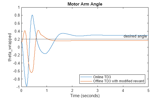
As expected, the TD3 agent trained offline does not drive the motor arm back to 0 because you change the desired angle from 0 to 0.2 rad in the new reward function. Note that online agent drives the motor arm to a position in which $\theta$ = 0.297 rad (instead of the front position in which $\theta$ = 0), despite $\theta$ being penalized with a negative reward. Similarly the offline agent drives the motor arm to a position in which $\theta$ =0.167 rad, (instead of the desired position $\theta$ = 0.2). More training or other modifications of the reward function could achieve a more precise behavior. For example, you can experiment with the weights of each term in the reward function.

Helper Functions

The function localEpisodeFinishedFcn selects the data that should be logged in every training episode. The function is used by the rlDataLogger object.

function dataToLog = localEpisodeFinishedFcn(data)
dataToLog = struct("data",data.Experience);
end

The function localResetFcn resets the initial angles to a random number and the intial speeds to 0. It is used by the Simulink environment.

function in = localResetFcn(in)
theta0 = -pi/4+rand*pi/2;
phi0 = pi-pi/4+rand*pi/2;
in = setVariable(in,"theta0",theta0);
in = setVariable(in,"phi0",phi0);
in = setVariable(in,"dtheta0",0);
in = setVariable(in,"dphi0",0);
end

The function localReadFcn reads experience data from the logged data files and modifies the reward of each experience. It is used by the fileDatastore object.

function experiences = localReadFcn(fileName)
data = load(fileName);
experiences = data.episodeData.data{:};
desired = 0.2; % desired angle
for idx = 1:numel(experiences)
    nextObs = experiences(idx).NextObservation;
    theta = atan2(nextObs{1}(1),nextObs{1}(2));
    newReward = ...
        experiences(idx).Reward - 0.1*(-2*desired*theta+desired^2);
    experiences(idx).Reward = newReward;
end
end

References

[1] Cazzolato, Benjamin Seth, and Zebb Prime. “On the Dynamics of the Furuta Pendulum.” Journal of Control Science and Engineering 2011 (2011): 1–8. https://doi.org/10.1155/2011/528341.