Credit Scorecard Validation Metrics
This example shows how to implement a probability of default (PD) model validation suite covering the techniques laid out in [1]. The techniques in [1] apply to any PD model. In this example, you load the test data, set and compute some key quantities, and calculate some model validation metrics. The results are stored in a collection object. You use the PDModel data set, which consists of a pre-fitted MATLAB® credit scorecard object. You then compute various metrics and summarize them.
Prepare Data
Load the scorecard to validate.
modelDataFile = "PDModel.mat";
inputData = load(modelDataFile);
Set the response variable and default indicator.
responseVar = "status";
outcomeIndicator = 1;
Extract key data and precompute certain key quantities.
sc = inputData.sc;
testData = sc.Data;
scores = sc.score;
defaultProbs = probdefault(sc);
defaultIndicators = testData.(responseVar) == outcomeIndicator;
Visualize Cumulative Accuracy Profile and Compute Accuracy Ratio
The cumulative accuracy profile (CAP) curve shows the proportion of defaulting names against the proportion of all names in the test set as the scores range from lower to higher values. The accuracy ratio (AR) measures how the model relates to hypothetical perfect and random models. An AR of 1 indicates the model is perfect, whereas an AR of 0 indicates the scoring model is no better than a random model.
Create a collection object for storing metrics.
MH = mrm.data.validation.MetricsHandler;
Calculate the CAP values and the AR. Plot the CAP curve.
CAPMetric = mrm.data.validation.pd.CAPAccuracyRatio(defaultIndicators,scores);
visualize(CAPMetric);
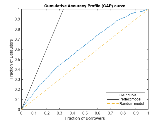
Display the accuracy ratio and append the CAP values to the collection object.
displayResult(CAPMetric);
Accuracy ratio is 0.3223
append(MH,CAPMetric);
Compute and Visualize Receiver Operating Characteristic
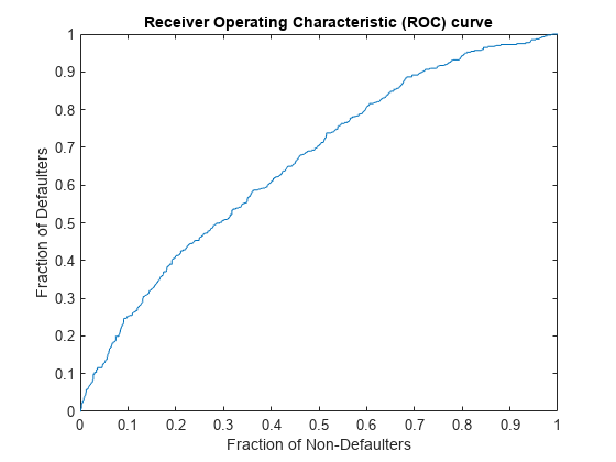
The receiver operating characteristic (ROC) curve shows the proportion of defaulting names against the proportion of non-defaulting names in the test set as the scores move from lower to higher values. The associated test metric is the area under the ROC curve (AUROC). An AUROC value of 1 indicates a perfect model.
Calculate the ROC values and plot the ROC curve.
ROCMetric = mrm.data.validation.pd.AUROC(defaultIndicators,scores);
visualize(ROCMetric);
Display the AUROC value and append the ROC values to the collection object.
displayResult(ROCMetric);
Area under ROC curve is 0.6611
append(MH,ROCMetric);
Compute and Visualize Kolmogorov-Smirnov Statistic
Calculate and plot the Kolmogorov-Smirnov statistic, which indicates the maximal separation of defaulters from non-defaulters that the model achieves. The two plots in the visualization are the fractions of defaulters and non-defaulters in the test set. Reference [1] refers to these quantities as the hit rate and the false alarm rate, respectively.
KSMetric = mrm.data.validation.pd.KSStatistic(defaultIndicators,scores);
visualize(KSMetric);

Display the Kolmogorov-Smirnov statistic and append the values to the collection object.
displayResult(KSMetric);
Kolmogorov-Smirnov statistic is 0.2232, at score 499.2
append(MH,KSMetric);
Compute and Visualize Pietra Index
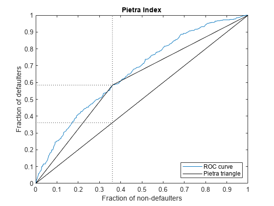
The Pietra Index is twice the maximal area of a triangle that can be fit between the ROC curve and the diagonal. Multiplication by 2 ensures that the range of possible values for the index is [0, 1].
Calculate and plot the Pietra Index. Assume that the area under the ROC is convex. In this case, the Pietra Index matches the Kolmogorov-Smirnov statistic, indicated by the vertical dotted line in the plot.
PietraMetric = mrm.data.validation.pd.PietraIndex(defaultIndicators,scores);
visualize(PietraMetric);
Display the Pietra metric and append it to the collection object.
displayResult(PietraMetric);
Pietra index is 0.2232
append(MH,PietraMetric);
Compute and Visualize Bayesian Error Rate
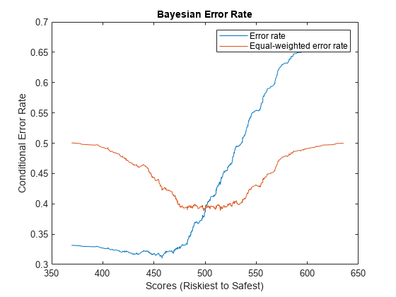
Define the error rate at a given score as this weighted sum:
,
where is the total proportion of defaulters in the test set, is the hit rate function, and is the false alarm rate function. The Bayesian error rate of the model is the minimum error rate in the test set. The error rate is sometimes calculated with equal weights of 0.5 instead of and . In this case the Bayesian error rate is equal to , where is the Kolmogorov-Smirnov statistic.
Calculate and plot the Bayesian error rate.
BERMetric = mrm.data.validation.pd.BayesianErrorRate(defaultIndicators,scores);
visualize(BERMetric);
Display the Bayesian error rate statistics in a table and append the values to a collection object.
displayResult(BERMetric);
                                           Value     Score
                                          _______    ______

    Bayesian error rate                      0.31     457.9
    Equal-weighted Bayesian error rate    0.38838    499.18
append(MH,BERMetric);
Calculate Mann-Whitney Statistic
The Mann-Whitney statistic is a rank sum metric that you calculate for the defaulter and non-defaulter populations of the test set. This metric recovers the AUROC statistic. You can use the variance of the Mann-Whitney statistic to calculate confidence intervals for the AUROC statistic.
Calculate the Mann-Whitney statistic, display the result, and append it to the collection object.
mwConfidenceLevel =0.95; MWMetric = mrm.data.validation.pd.MannWhitneyMetric(defaultIndicators,scores, ... mwConfidenceLevel); displayResult(MWMetric);
Mann-Whitney statistic 0.66113, with confidence interval (0.6606,0.66165) at level 0.95
append(MH,MWMetric);
Calculate Somers' D Value
To test the hypothesis that a low score correspond to a high probability of default, calculate the Somers' D between the sorted scores and the default indicators (flipped, to preserve the ordering, so that survival is denoted by 1 and default by 0).
SDMetric = mrm.data.validation.pd.SomersDMetric(defaultIndicators,scores);
displayResult(SDMetric);
Somers' D is 0.3223
append(MH,SDMetric)
Display Brier Score
The Brier score is the mean squared error of the probabilities of default that the model predicts. Calculate the Brier score also for the model that assigns the same probability to each name (equal to the fraction of defaulting names in the data set). Display the result and append it to the collection object.
BrierMetric = mrm.data.validation.pd.BrierTestMetric(defaultIndicators,defaultProbs);
displayResult(BrierMetric);
                                      Value
                                     _______

    Brier score                      0.20541
    Brier score for trivial model    0.22138
append(MH,BrierMetric);
Perform Binomial Test
The binomial test inspects each rating category separately and tests whether the number of realized defaults is plausible for the predicted probability of default.
Set the confidence level using the q variable. For example, to calculate the scores at which the number of observed defaults exceeds the expected defaults with 95% confidence, set q to 0.95. Divide the scores into ratings categories using the discretize function. Plot the test results. Any observed defaults that are in excess of the maximal expected number are highlighted with an asterisk.
q = 0.95;
ratings = discretize(scores,15);
BinMetric = mrm.data.validation.pd.BinomialTest(defaultIndicators,defaultProbs,scores,q,ratings);
visualize(BinMetric);
0.95;
ratings = discretize(scores,15);
BinMetric = mrm.data.validation.pd.BinomialTest(defaultIndicators,defaultProbs,scores,q,ratings);
visualize(BinMetric);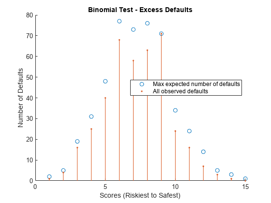
Display the test results in a table and append the metric to the collection object.
head(formatResult(BinMetric));
    Rating Category    Observed Defaults    Max Expected Number of Defaults
    _______________    _________________    _______________________________

           1                   1                           2
           2                   4                           5
           3                  16                          19
           4                  25                          31
           5                  40                          48
           6                  68                          77
           7                  58                          73
           8                  63                          76
append(MH,BinMetric);
Compute Hosmer-Lemeshow Metric
The Hosmer-Lemeshow metric, also known as the chi-square test, compares the number of observed defaults for each ratings category with the expected number from the probability of default that the model predicts. Unlike the results of the binomial test, these measures are combined into a single quantity, which for large data sets converges to a -distribution, where is the number of rating categories in the model. The test statistic is the -value of this -distribution.
HLMetric = mrm.data.validation.pd.HosmerLemeshowMetric(defaultIndicators,defaultProbs,scores);
displayResult(HLMetric);
Hosmer-Lemeshow p-value is 0.9177
append(MH,HLMetric);
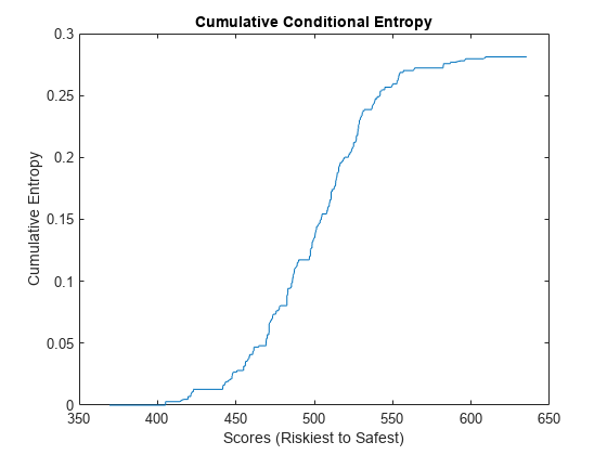
Compute and Visualize Entropy Measures
The conditional information entropy ratio (CIER) measures the capability of the model to separate defaulters from non-defaulters. Unlike the other metrics you calculate in this example, the CIER does not depend on the ordering of the scores. A CIER value close to zero indicates good separation of defaulting names from surviving names.
Calculate and plot the CIER. The plot shows the cumulative sum of the entropies at each score weighted by the proportion of names with that score. Jumps indicate points at which the model struggles to differentiate between defaulters and non-defaulters.
CIERMetric = mrm.data.validation.pd.EntropyMetric(defaultIndicators,scores);
visualize(CIERMetric);
Display the CIER and append the statistics to the collection object.
displayResult(CIERMetric);
Conditional Information Entropy Ratio is 0.557
append(MH,CIERMetric);
Display Summary
Display a summary of the calculated statistics for the example model.
disp(report(MH))
                    Metric                      Value
    _______________________________________    _______

    "Accuracy ratio"                           0.32225
    "Area under ROC curve"                     0.66113
    "Kolmogorov-Smirnov statistic"             0.22324
    "Pietra index"                             0.22324
    "Bayesian error rate"                         0.31
    "Mann-Whitney u-test"                      0.66113
    "Somers' D"                                0.32225
    "Brier score"                              0.20541
    "Binomial test failure rate"                     0
    "Hosmer-Lemeshow p-value"                  0.91772
    "Conditional Information Entropy Ratio"    0.55697
References
[1] Basel Committee on Banking Supervision, Working Paper 14. "Studies on the Validation of Internal Rating Systems (revised)." Bank for International Settlements. https://www.bis.org/publ/bcbs_wp14.htm.