Coverage Maps for Satellite Constellation
This example shows how to display coverage maps for a region of interest using a satellite scenario and 2-D maps. A coverage map for satellites includes received power over an area for a downlink to ground-based receivers within the area.
By combining the mapping capabilities in Mapping Toolbox™ with the satellite scenario capabilities in Satellite Communications Toolbox, you can create contoured coverage maps and use the contour data for visualization and analysis. This example shows you how to:
Compute coverage map data using a satellite scenario containing a grid of ground station receivers.
View coverage maps using different map displays, including
axesm-based maps and map axes.Compute and view coverage maps for other times of interest.
Create and Visualize Scenario
Create a satellite scenario and a viewer. Specify the start date and duration of 1 hour for the scenario.
startTime = datetime(2023,2,21,18,0,0);
stopTime = startTime + hours(1);
sampleTime = 60; % seconds
sc = satelliteScenario(startTime,stopTime,sampleTime);
viewer = satelliteScenarioViewer(sc,ShowDetails=false);
Add Satellite Constellation
The Iridium NEXT satellite network, launched between 2018 and 2019 [1], contains 66 active LEO satellites with:
Six orbital planes with an approximate inclination of 86.6 degrees and difference of RAAN of approximately 30 degrees between planes [1].
11 satellites per orbital plane with an approximate difference in true anomaly of 32.7 degrees between satellites [1].
Add the active Iridium NEXT satellites to the scenario. Create the orbital elements for the satellites in the Iridium network and create the satellites.
numSatellitesPerOrbitalPlane = 11;
numOrbits = 6;

orbitIdx = repelem(1:numOrbits,1,numSatellitesPerOrbitalPlane);
planeIdx = repmat(1:numSatellitesPerOrbitalPlane,1,numOrbits);

RAAN = 180*(orbitIdx-1)/numOrbits;
trueanomaly = 360*(planeIdx-1 + 0.5*(mod(orbitIdx,2)-1))/numSatellitesPerOrbitalPlane;
semimajoraxis = repmat((6371 + 780)*1e3,size(RAAN)); % meters
inclination = repmat(86.4,size(RAAN)); % degrees
eccentricity = zeros(size(RAAN)); % degrees
argofperiapsis = zeros(size(RAAN)); % degrees

iridiumSatellites = satellite(sc,...
    semimajoraxis,eccentricity,inclination,RAAN,argofperiapsis,trueanomaly,...
    Name="Iridium " + string(1:66)');
If you have a license for Aerospace Toolbox, you can also create the Iridium constellation using the walkerStar (Aerospace Toolbox) function.
Define Area of Interest Surrounding Australia
Prepare to compute the coverage map by creating an area of interest (AOI) surrounding Australia.
Read a shapefile containing world land areas into the workspace as a geospatial table. The geospatial table represents the land areas using polygon shapes in geographic coordinates. Extract the polygon shape for Australia.
landareas = readgeotable("landareas.shp");
australia = geocode("Australia",landareas);
Create a new polygon shape in geographic coordinates that includes a buffer region of 1 degree around the Australian land area. The buffer ensures the coverage map extents can cover the land area.
bufwidth = 1; % degrees
aoi = buffer(australia.Shape,bufwidth);
Add Grid of Ground Stations Covering AOI
Create the coverage map data by computing signal strength for a grid of ground station receivers covering the AOI. Create ground station locations by creating a grid of latitude-longitude coordinates and selecting the coordinates within the AOI.
Compute latitude and longitude limits for the AOI and specify a spacing in degrees. The spacing determines the distance between the ground stations. A lower spacing value results in improved coverage map resolution but also increases computation time.
[latlim, lonlim] = bounds(aoi);
spacingInLatLon = 1; % degrees
Create a projected coordinate reference system (CRS) that is appropriate for Australia. A projected CRS provides information that assigns Cartesian x and y map coordinates to physical locations. Use the GDA2020 / GA LCC projected CRS appropriate for Australia that uses the Lambert Conformal Conic projection.
proj = projcrs(7845);
Calculate the projected X-Y map coordinates for the data grid. Use the projected X-Y map coordinates instead of latitude-longitude coordinates to reduce variation in the distance between grid locations.
spacingInXY = deg2km(spacingInLatLon)*1000; % meters
[xlimits,ylimits] = projfwd(proj,latlim,lonlim);
R = maprefpostings(xlimits,ylimits,spacingInXY,spacingInXY);
[X,Y] = worldGrid(R);
Transform the grid locations to latitude-longitude coordinates.
[gridlat,gridlon] = projinv(proj,X,Y);
Select the grid coordinates within the AOI.
gridpts = geopointshape(gridlat,gridlon);
inregion = isinterior(aoi,gridpts);

gslat = gridlat(inregion);
gslon = gridlon(inregion);
Create ground stations for the coordinates.
gs = groundStation(sc,gslat,gslon);
Add Transmitters and Receivers
Enable the modeling of downlinks by adding transmitters to the satellites and adding receivers to the ground stations.
The Iridium constellation uses a 48-beam antenna. Select a Gaussian antenna or a custom 48-beam antenna (Phased Array System Toolbox™ required) or a measuredAntenna (Antenna Toolbox™ required). The Gaussian antenna approximates the 48-beam antenna by using the Iridium half view angle of 62.7 degrees [1]. Orient the antenna to point towards the nadir direction.
fq = 1625e6; % Hz txpower = 20; % dBW antennaType ="Gaussian"; halfBeamWidth = 62.7; % degrees
Add satellite transmitters with Gaussian antennas.
if antennaType == "Gaussian"
    lambda = physconst('lightspeed')/fq; % meters
    dishD = (70*lambda)/(2*halfBeamWidth); % meters
    tx = transmitter(iridiumSatellites, ...
        Frequency=fq, ...
        Power=txpower);
    gaussianAntenna(tx,DishDiameter=dishD);
end
Add satellite transmitters with custom 48-beam antenna. The helper function helperCustom48BeamAntenna is included with the example as a supporting file.
if antennaType == "Custom 48-Beam"
    antenna = helperCustom48BeamAntenna(fq);
    tx = transmitter(iridiumSatellites, ...
        Frequency=fq, ...
        MountingAngles=[0,-90,0], ... % [yaw, pitch, roll] with -90 using Phased Array System Toolbox convention
        Power=txpower, ...
        Antenna=antenna);
end
Add satellite transmitters using the measuredAntenna object, which accepts the measured or simulated directivity values of an user designed antenna. The measured or simulated pattern data must include the directivity values, the direction in which the values are measured or simulated, and the corresponding azimuth and elevation angles. You can import this data into workspace using any MATLAB-supported file format. This example uses radiation pattern data from the attached patternData.csv file. Read the CSV-file which contains the azimuth, elevation and directivity values. The direction value is populated using the azimuth, elevation values obtained from the file and the farfield distance as first, second and third column respectively. Create a measuredAntenna object and set its Directivity, Direction, Azimuth, and Elevation properties.
if antennaType == "Measured Antenna"
    patData = readmatrix("patternData.csv");

    lambda = physconst("LightSpeed")/fq; % meters
    R = 100*lambda;
    direction = [patData(:,1) patData(:,2) R*ones(numel(patData(:,1)),1)];   % Direction values [azimuth,elevation,farfield distance]
    azimuth = unique(patData(:,1));
    elevation = unique(patData(:,2));

    antenna = measuredAntenna(Directivity = patData(:,3),...
        Direction = direction,Azimuth = azimuth,Elevation = elevation,E = [],FieldFrequency = fq);

    tx = transmitter(iridiumSatellites, ...
        Frequency=fq, ...
        Power=txpower,...
        Antenna = antenna);
end
Add Ground Station Receivers
Add ground station receivers with isotropic antennas.
isotropic = arrayConfig(Size=[1 1]);
rx = receiver(gs,Antenna=isotropic);
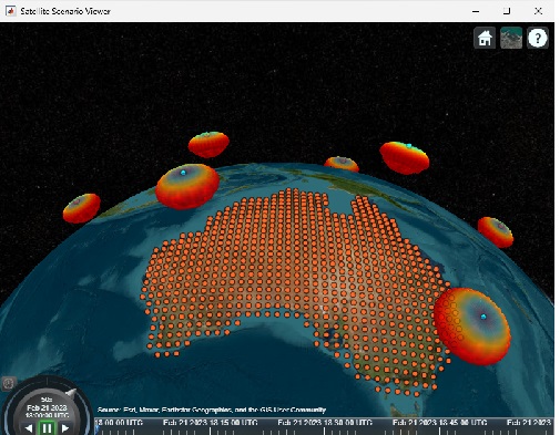
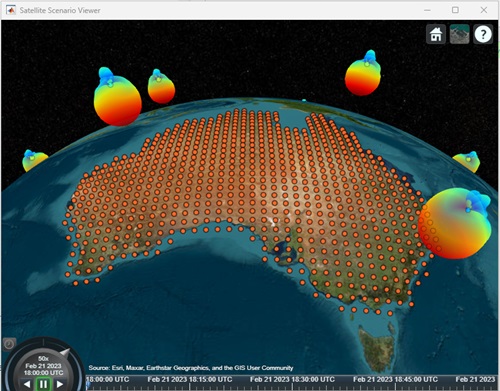
Visualize the satellite transmitter antenna patterns. The visualization shows the nadir-pointing orientation of the antennas.
pattern(tx,Size=500000);
Gaussian Antenna

Custom 48-Beam
Measured Antenna
Compute Raster Coverage Map Data
Close satellite scenario viewer and compute coverage data corresponding to the scenario start time. The satcoverage helper function returns gridded coverage data. For each satellite, the function computes a field-of-view shape and calculates signal strength for each ground station receiver within the satellite field-of-view. The coverage data is the maximum signal strength received from any satellite.
delete(viewer)
maxsigstrength = satcoverage(gridpts,sc,startTime,inregion,halfBeamWidth);
Visualize Coverage on an axesm-Based Map
Plot the raster coverage map data on an axesm-based map corresponding to Australia. An axesm-based map is used because the geoshow function can create contour plots from matrix data, whereas map axes require you to manually contour the data.
Define minimum and maximum power levels for the display.
minpowerlevel = -120; % dBm
maxpowerlevel = -106; % dBm
Create a world map for Australia and plot the raster coverage map data as a contour display.
figure
worldmap(latlim,lonlim)
mlabel south

colormap turbo
clim([minpowerlevel maxpowerlevel])
geoshow(gridlat,gridlon,maxsigstrength,DisplayType="contour",Fill="on")
geoshow(australia,FaceColor="none")

cBar = contourcbar;
title(cBar,"dBm");
title("Signal Strength at " + string(startTime) + " UTC")
Add text labels for the cities of Sydney, Melbourne, and Brisbane. Get the coordinates of each city by using the geocode function.
sydneyT = geocode("Sydney,Australia","city");
sydney = sydneyT.Shape;
melbourneT = geocode("Melbourne,Australia","city");
melbourne = melbourneT.Shape;
brisbaneT = geocode("Brisbane,Australia","city");
brisbane = brisbaneT.Shape;

textm(sydney.Latitude,sydney.Longitude,"Sydney")
textm(melbourne.Latitude,melbourne.Longitude,"Melbourne")
textm(brisbane.Latitude,brisbane.Longitude,"Brisbane")

Custom 48-Beam

Measured Antenna

Compute Coverage Map Contours
Contour the raster coverage map data to create a geospatial table of coverage map contours. Each coverage map contour is represented as a row in the geospatial table containing a polygon shape in geographic coordinates. You can use the coverage map contours for both visualization and analysis.
levels = linspace(minpowerlevel,maxpowerlevel,8);
GT = contourDataGrid(gridlat,gridlon,maxsigstrength,levels,proj);
GT = sortrows(GT,"Power (dBm)");
disp(GT)
Shape Area (sq km) Power (dBm) Power Range (dBm)
____________ ____________ ___________ _________________
geopolyshape 8.5438e+06 -120 -120 -118
geopolyshape 8.2537e+06 -118 -118 -116
geopolyshape 5.5606e+06 -116 -116 -114
geopolyshape 3.6841e+06 -114 -114 -112
geopolyshape 2.2841e+06 -112 -112 -110
geopolyshape 1.1843e+06 -110 -110 -108
geopolyshape 3.8306e+05 -108 -108 -106
Custom 48-Beam

Measured Antenna

Visualize Coverage on a Map Axes
Plot the coverage map contours on a map axes using the map projection corresponding to Australia. For more information, see Choose a 2-D Map Display (Mapping Toolbox).
figure
newmap(proj)
hold on

colormap turbo
clim([minpowerlevel maxpowerlevel])
geoplot(GT,ColorVariable="Power (dBm)",EdgeColor="none")
geoplot(australia,FaceColor="none")

cBar = colorbar;
title(cBar,"dBm");
title("Signal Strength at " + string(startTime) + " UTC")

text(sydney.Latitude,sydney.Longitude,"Sydney",HorizontalAlignment="center")
text(melbourne.Latitude,melbourne.Longitude,"Melbourne",HorizontalAlignment="center")
text(brisbane.Latitude,brisbane.Longitude,"Brisbane",HorizontalAlignment="center")

Custom 48-Beam

Measured Antenna

Compute and Visualize Coverage for Different Time of Interest
Specify a different time of interest and compute and visualize coverage.
secondTOI = startTime + minutes(2); % 2 minutes after the start of the scenario
maxsigstrength = satcoverage(gridpts,sc,secondTOI,inregion,halfBeamWidth);

GT2 = contourDataGrid(gridlat,gridlon,maxsigstrength,levels,proj);
GT2 = sortrows(GT2,"Power (dBm)");

figure
newmap(proj)
hold on

colormap turbo
clim([minpowerlevel maxpowerlevel])
geoplot(GT2,ColorVariable="Power (dBm)",EdgeColor="none")
geoplot(australia,FaceColor="none")

cBar = colorbar;
title(cBar,"dBm");
title("Signal Strength at " + string(secondTOI) + " UTC")

text(sydney.Latitude,sydney.Longitude,"Sydney",HorizontalAlignment="center")
text(melbourne.Latitude,melbourne.Longitude,"Melbourne",HorizontalAlignment="center")
text(brisbane.Latitude,brisbane.Longitude,"Brisbane",HorizontalAlignment="center")

Custom 48-Beam

Measured Antenna

Compute Coverage Levels for Cities
Compute and display coverage levels for three cities in Australia.
covlevels1 = [coveragelevel(sydney,GT); coveragelevel(melbourne,GT); coveragelevel(brisbane,GT)];
covlevels2 = [coveragelevel(sydney,GT2); coveragelevel(melbourne,GT2); coveragelevel(brisbane,GT2)];

covlevels = table(covlevels1,covlevels2, ...
RowNames=["Sydney" "Melbourne" "Brisbane"], ...
VariableNames=["Signal Strength at T1 (dBm)" "Signal Strength T2 (dBm)"])
covlevels=3×2 table
                 Signal Strength at T1 (dBm)    Signal Strength T2 (dBm)
                 ___________________________    ________________________

    Sydney                  -108                          -112
    Melbourne               -112                          -110
    Brisbane                -112                          -116
Custom 48-Beam

Measured Antenna

Helper Functions
The satcoverage helper function returns coverage data. For each satellite, the function computes a field-of-view shape and calculates signal strength for each ground station receiver within the satellite field-of-view. The coverage data is the maximum signal strength received from any satellite.
function coveragedata = satcoverage(gridpts,sc,timeIn,inregion,halfBeamWidth)

    % Get satellites and ground station receivers
    sats = sc.Satellites;
    rxs = [sc.GroundStations.Receivers];

    % Get field-of-view shapes for all satellites
    fovs = satfov(sats,timeIn,halfBeamWidth);

    % Initialize coverage data
    coveragedata = NaN(size(gridpts));

    for satind = 1:numel(sats)
        fov = fovs(satind);

        % Find grid and rx locations which are within the satellite field-of-view
        gridInFOV = isinterior(fov,gridpts);
        rxInFOV = gridInFOV(inregion);

        % Compute sigstrength at grid locations using temporary link objects
        gridsigstrength = NaN(size(gridpts));
        if any(rxInFOV)
            tx = sats(satind).Transmitters;
            lnks = link(tx,rxs(rxInFOV));
            rxsigstrength = sigstrength(lnks,timeIn)+30; % Convert from dBW to dBm
            gridsigstrength(inregion & gridInFOV) = rxsigstrength;
            delete(lnks)
        end

        % Update coverage data with maximum signal strength found
        coveragedata = max(gridsigstrength,coveragedata);
    end
end
The satfov helper function returns an array of geopolyshape objects representing the field-of-view for each satellite, assuming nadir-pointing and a spherical Earth model.
function fovs = satfov(sats,timeIn,halfViewAngle)

    % Compute the latitude, longitude, and altitude of all satellites at the input time
    satstates = states(sats,timeIn,CoordinateFrame="geographic");

    fovs = createArray([1 numel(sats)],"geopolyshape");
    for satind = 1:numel(sats)
        lla = satstates(:,1,satind);

        % Find the Earth central angle using the beam view angle
        if isreal(acosd(sind(halfViewAngle)*(lla(3)+earthRadius)/earthRadius))
            % Case when Earth FOV is bigger than antenna FOV
            earthCentralAngle = 90-acosd(sind(halfViewAngle)*(lla(3)+earthRadius)/earthRadius)-halfViewAngle;
        else
            % Case when antenna FOV is bigger than Earth FOV
            earthCentralAngle = 90-halfViewAngle;
        end

        % Create a circular geopolyshape centered at the position of the satellite
        % with a buffer of width equaling the Earth central angle
        fovs(satind) = aoicircle(lla(1),lla(2),earthCentralAngle);
    end
end
The contourDataGrid helper function contours a data grid and returns the result as a geospatial table. Each row of the table corresponds to a power level and includes the contour shape, the area of the contour shape in square kilometers, the minimum power for the level, and the power range for the level.
function GT = contourDataGrid(latd,lond,data,levels,proj)

    % Pad each side of the grid to ensure no contours extend past the grid bounds
    lond = [2*lond(1,:)-lond(2,:); lond; 2*lond(end,:)-lond(end-1,:)];
    lond = [2*lond(:,1)-lond(:,2) lond 2*lond(:,end)-lond(:,end-1)];
    latd = [2*latd(1,:)-latd(2,:); latd; 2*latd(end,:)-latd(end-1,:)];
    latd = [2*latd(:,1)-latd(:,2) latd 2*latd(:,end)-latd(:,end-1)];
    data = [ones(size(data,1)+2,1)*NaN [ones(1,size(data,2))*NaN; data; ones(1,size(data,2))*NaN] ones(size(data,1)+2,1)*NaN];

    % Replace NaN values in power grid with a large negative number
    data(isnan(data)) = min(levels) - 1000;

    % Project the coordinates using an equal-area projection
    [xd,yd] = projfwd(proj,latd,lond);

    % Contour the projected data
    fig = figure("Visible","off");
    obj = onCleanup(@()close(fig));
    c = contourf(xd,yd,data,LevelList=levels);

    % Initialize variables
    x = c(1,:);
    y = c(2,:);
    n = length(y);
    k = 1;
    index = 1;
    levels = zeros(n,1);
    latc = cell(n,1);
    lonc = cell(n,1);

    % Process the coordinates of the projected contours
    while k < n
        level = x(k);
        numVertices = y(k);
        yk = y(k+1:k+numVertices);
        xk = x(k+1:k+numVertices);
        k = k + numVertices + 1;

        [first,last] = findNanDelimitedParts(xk);
        jindex = 0;
        jy = {};
        jx = {};

        for j = 1:numel(first)
            % Process the j-th part of the k-th level
            s = first(j);
            e = last(j);
            cx = xk(s:e);
            cy = yk(s:e);
            if cx(end) ~= cx(1) && cy(end) ~= cy(1)
                cy(end+1) = cy(1); %#ok<*AGROW>
                cx(end+1) = cx(1);
            end

            if j == 1 && ~ispolycw(cx,cy)
                % First region must always be clockwise
                [cx,cy] = poly2cw(cx,cy);
            end

            % Filter regions made of collinear points or fewer than 3 points
            if ~(length(cx) < 4 || all(diff(cx) == 0) || all(diff(cy) == 0))
                jindex = jindex + 1;
                jy{jindex,1} = cy(:)';
                jx{jindex,1} = cx(:)';
            end
        end

        % Unproject the coordinates of the processed contours
        [jx,jy] = polyjoin(jx,jy);
        if length(jy) > 2 && length(jx) > 2
            [jlat,jlon] = projinv(proj,jx,jy);
            latc{index,1} = jlat(:)';
            lonc{index,1} = jlon(:)';
            levels(index,1) = level;
            index = index + 1;
        end
    end

    % Create contour shapes from the unprojected coordinates. Include the
    % contour shapes, the areas of the shapes, and the power levels in a
    % geospatial table.
    latc = latc(1:index-1);
    lonc = lonc(1:index-1);
    Shape = geopolyshape(latc,lonc);

    Area = area(Shape);

    levels = levels(1:index-1);
    Levels = levels;

    allPartsGT = table(Shape,Area,Levels);

    % Condense the geospatial table into a new geospatial table with one
    % row per power level.
    GT = table.empty;
    levels = unique(allPartsGT.Levels);
    for k = 1:length(levels)
        gtLevel = allPartsGT(allPartsGT.Levels == levels(k),:);
        tLevel = geotable2table(gtLevel,["Latitude","Longitude"]);
        [lon,lat] = polyjoin(tLevel.Longitude,tLevel.Latitude);
        Shape = geopolyshape(lat,lon);
        Levels = levels(k);
        Area = area(Shape);
        GT(end+1,:) = table(Shape,Area,Levels);
    end

    maxLevelDiff = max(abs(diff(GT.Levels)));
    LevelRange = [GT.Levels GT.Levels + maxLevelDiff];
    GT.LevelRange = LevelRange;

    % Clean up the geospatial table
    GT.Area = GT.Area/1e6;
    GT.Properties.VariableNames = ...
        ["Shape","Area (sq km)","Power (dBm)","Power Range (dBm)"];
end
The coveragelevel function returns the coverage level for a geopointshape object.
function powerLevels = coveragelevel(point,GT)

    % Determine whether points are within coverage
    inContour = false(length(GT.Shape),1);
    for k = 1:length(GT.Shape)
        inContour(k) = isinterior(GT.Shape(k),point);
    end

    % Find the highest coverage level containing the point
    powerLevels = max(GT.("Power (dBm)")(inContour));

    % Return -inf if the point is not contained within any coverage level
    if isempty(powerLevels)
        powerLevels = -inf;
    end
end
The findNanDelimitedParts helper function finds the indices of the first and last elements of each NaN-separated part of the array x.
function [first,last] = findNanDelimitedParts(x)

    % Find indices of the first and last elements of each part in x.
    % x can contain runs of multiple NaNs, and x can start or end with
    % one or more NaNs.

    n = isnan(x(:));

    firstOrPrecededByNaN = [true; n(1:end-1)];
    first = find(~n & firstOrPrecededByNaN);

    lastOrFollowedByNaN = [n(2:end); true];
    last = find(~n & lastOrFollowedByNaN);
end
References
[1] Attachment EngineeringStatement SAT-MOD-20131227-00148. https://fcc.report/IBFS/SAT-MOD-20131227-00148/1031348. Accessed 17 Jan. 2023.
See Also
aoicircle (Mapping Toolbox)
Topics
- Read Quantitative Data from WMS Server (Mapping Toolbox)