detect

Detect anomalies in signals

Since R2023a

Syntax

[lbls,loss] = detect(d,data)

[lbls,loss] = detect(d,data,Name=Value)

Description

[lbls,loss] = detect(d,data) detects anomalies in signals stored in data.

The function assigns a normal label to signal windows whose aggregated loss value is below the detection threshold, and an abnormal label to signal windows whose aggregated loss value is greater than or equal to the detection threshold.

[lbls,loss] = detect(d,data,Name=Value) specifies additional options using name-value arguments.

Examples

Detect Sinusoid Anomalies with Trained Autoencoder

Load a convolutional anomaly detector trained with three-channel sinusoidal signals. Display the model, threshold, and window properties of the detector.

load sineWaveAnomalyDetector
D

D = 
  deepSignalAnomalyDetectorCNN with properties:

                IsTrained: 1
              NumChannels: 3

   Model Information
                ModelType: 'convautoencoder'
               FilterSize: 8
               NumFilters: 32
      NumDownsampleLayers: 2
         DownsampleFactor: 2
       DropoutProbability: 0.2000

   Threshold Information
                Threshold: 0.0510
          ThresholdMethod: 'contaminationFraction'
       ThresholdParameter: 0.0100

   Window Information
             WindowLength: 1
            OverlapLength: 'auto'
    WindowLossAggregation: 'mean'

Load the file sineWaveAnomalyData.mat, which contains two sets of synthetic three-channel sinusoidal signals.

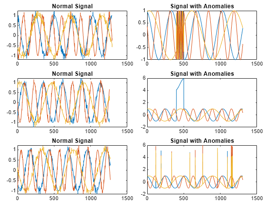
• sineWaveNormal contains the 10 sinusoids used to train the convolutional anomaly detector. Each signal has a series of small-amplitude impact-like imperfections but otherwise has stable amplitude and frequency.

• sineWaveAbnormal contains three signals of similar length and amplitude to the training data. One of the signals has an abrupt, finite-time change in frequency. Another signal has a finite-duration amplitude change in one of its channels. A third has random spikes in each channel.

Plot three normal signals and the three signals with anomalies.

load sineWaveAnomalyData

tiledlayout(3,2,TileSpacing="compact",Padding="compact")
rnd = randperm(length(sineWaveNormal));
for kj = 1:3
    nexttile
    plot(sineWaveNormal{rnd(kj)})
    title("Normal Signal")
    nexttile
    plot(sineWaveAbnormal{kj})
    title("Signal with Anomalies")
end

Use the trained anomaly detector to detect the anomalies in the abnormal data.

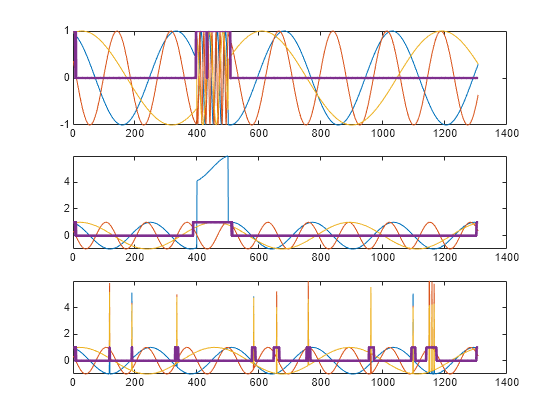
[lbls,loss] = detect(D,sineWaveAbnormal);

The first output of detect is a categorical array that declares each sample of a signal as being anomalous or not.

tiledlayout("vertical")
for kj = 1:3
    nexttile
    plot(sineWaveAbnormal{kj})
    hold on
    plot(lbls{kj},LineWidth=2)
end

Detect Anomalies in Streaming Sinusoids

Load the file sineWaveAnomalyData.mat, which contains two sets of synthetic three-channel sinusoidal signals.

• sineWaveNormal contains the 10 sinusoids used to train the convolutional anomaly detector. Each signal has a series of small-amplitude impact-like imperfections but otherwise has stable amplitude and frequency.

• sineWaveAbnormal contains three signals of similar length and amplitude to the training data. One of the signals has an abrupt, finite-time change in frequency. Another signal has a finite-duration amplitude change in one of its channels. A third has random spikes in each channel.

Plot three normal signals and the three signals with anomalies.

load sineWaveAnomalyData
 
tiledlayout(3,2,TileSpacing="compact",Padding="compact")
rnd = randperm(length(sineWaveNormal));
for kj = 1:length(sineWaveAbnormal)
    nexttile
    plot(sineWaveNormal{rnd(kj)})
    title("Normal Signal")
    nexttile
    plot(sineWaveAbnormal{kj})
    title("Signal with Anomalies")
end

Create a long short-term memory (LSTM) forecaster object to detect the anomalies in the abnormal signals. Specify a window length of 10 samples.

D = deepSignalAnomalyDetector(3,"lstmforecaster",windowLength=10);

Train the forecaster using the anomaly-free sinusoids. Use the training options for the adaptive moment estimation (Adam) optimizer and specify a maximum number of 100 epochs. For more information, see trainingOptions (Deep Learning Toolbox).

opts = trainingOptions("adam",MaxEpochs=100,ExecutionEnvironment="cpu");
trainDetector(D,sineWaveNormal,opts)

    Iteration    Epoch    TimeElapsed    LearnRate    TrainingLoss
    _________    _____    ___________    _________    ____________
            1        1       00:00:01        0.001          0.6369
           50       50       00:00:08        0.001         0.19706
          100      100       00:00:17        0.001        0.064225
Training stopped: Max epochs completed
Computing threshold...
Threshold computation completed.

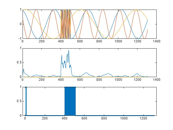
Use the trained detector to find the anomalies in the first signal. Reset the state of the detector. Stream the data one sample at a time and have the detector keep its state after each reading. Compute the reconstruction loss for each one-sample frame. Categorize signal regions where the loss exceeds a specified threshold as anomalous.

resetState(D)

sg = sineWaveAbnormal{1};
anoms = NaN(size(sg));
losss = zeros(size(sg));

for kj = 1:length(sg)
    frame = sg(kj,:);
    [lb,lo] = detect(D,frame, ...
        KeepState=true,ExecutionEnvironment="cpu");
    anoms(kj) = lb;
    losss(kj) = lo;
end

Plot the anomalous signal, the reconstruction loss, and the categorical array that declares each sample of the signal as being anomalous or not.

figure
tiledlayout("vertical")
nexttile
plot(sg)
nexttile
plot(losss)
nexttile
stem(anoms,".")

Reset the state of the detector. Find the anomalies in the third signal. Plot the anomalous signal, the reconstruction loss, and the categorical array that declares each sample of the signal as being anomalous or not.

resetState(D)

sg = sineWaveAbnormal{3};
anoms = NaN(size(sg));
losss = zeros(size(sg));

for kj = 1:length(sg)
    frame = sg(kj,:);
    [lb,lo] = detect(D,frame, ...
        KeepState=true,ExecutionEnvironment="cpu");
    anoms(kj) = lb;
    losss(kj) = lo;
end

figure
tiledlayout("vertical")
nexttile
plot(sg)
nexttile
plot(losss)
nexttile
stem(anoms,".")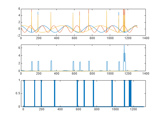

Input Arguments

d — Anomaly detector

deepSignalAnomalyDetectorCNN object | deepSignalAnomalyDetectorLSTM object | deepSignalAnomalyDetectorLSTMForecaster object

Anomaly detector, specified as a deepSignalAnomalyDetectorCNN object, a deepSignalAnomalyDetectorLSTM object, or a deepSignalAnomalyDetectorLSTMForecaster object. Use the deepSignalAnomalyDetector function to create d.

data — Signal data set

N_c-column matrix | M-element cell array | timetable | datastore

Signal data set, specified as one of these:

• N_c-column matrix — A single multichannel signal observation (M = 1), where N_c is equal to the value of the NumChannels property of the detector.

• M-element cell array — M multichannel signal observations, where each cell contains an N_c-column matrix.

• Timetable — A single multichannel signal observation, contained in a MATLAB^® timetable. The timetable must contain increasing, uniformly-sampled, and finite values. The timetable can have:

  • A single variable containing an N_c-column matrix, where each column corresponds to a signal channel.

  • N_c variables, where each variable contains a vector that corresponds to a signal channel.

• Datastore — A signalDatastore, audioDatastore (Audio Toolbox), or arrayDatastore object. The detector uses the readall function to read all the signal observations contained in the datastore at once. You can also use a CombinedDatastore or TransformedDatastore object containing any of the supported datastores.

Name-Value Arguments

Specify optional pairs of arguments as Name1=Value1,...,NameN=ValueN, where Name is the argument name and Value is the corresponding value. Name-value arguments must appear after other arguments, but the order of the pairs does not matter.

Example: MiniBatchSize=64,ExecutionEnvironment="cpu" instructs the function to use a mini-batch size of 64 and use the computer CPU to detect anomalies.

ExpandWindowLabels — Option to expand window labels

false (default) | true

Option to expand window labels to each sample, specified as either false or true.

• If you specify ExpandWindowLabels as false, then lbls contains one label per window.

• If you specify ExpandWindowLabels as true, then lbls contains one label per sample.

Data Types: logical

OverlapPriority — Label priority for overlapped windows

"anomaly" (default) | "normal"

Label priority for overlapped windows when ExpandWindowLabels is true, specified as "anomaly" or "normal".

• If you specify OverlapPriority as "anomaly", the function labels samples in an abnormal window overlapped with a normal window as abnormal.

• If you specify OverlapPriority as "normal", the function labels samples in a normal window overlapped with an abnormal window as normal.

This argument applies only when you set ExpandWindowLabels is true and the window overlap length is greater than zero.

Data Types: char | string

KeepState — Option to keep internal states

false (default) | true

Since R2024a

Option to keep the internal states of the anomaly detector so they persist during subsequent calls to detect, specified as false or true. Specify this argument as true when processing a continuous signal across multiple calls to ensure that the model incorporates historical data.

KeepState can be true only when:

• ModelType is "lstmforecaster".

• WindowLength is a number. fullSignal is not supported.

• OverlapLength is equal to WindowLength – 1.

• data has a batch size greater than 1.

Data Types: logical

MiniBatchSize — Mini-batch size

128 (default) | positive integer scalar

Mini-batch size used by the network to compute reconstructed signals, specified as a positive integer scalar.

Data Types: single | double | int8 | int16 | int32 | int64 | uint8 | uint16 | uint32 | uint64

ExecutionEnvironment — Execution environment

"auto" (default) | "gpu" | "cpu"

Execution environment used by the network, specified as one of these:

• "auto" — If available, use the GPU. If the GPU is not available, use the CPU.

• "gpu" — Use the GPU.

• "cpu" — Use the CPU.

Data Types: char | string

Output Arguments

lbls — Labels

logical column vector | cell array | timetable

Labels, returned as a logical column vector, cell array, or timetable. The output format of lbls depends on the format of data.

• If data is an N_c-column matrix, then lbls is a logical column vector.

• If data is an M-element cell array, then lbls is a cell array containing M logical column vectors.

• If data is a timetable, then lbls is a timetable with a single variable containing a logical column vector.

• If data is a datastore, then lbls is a vector or cell array depending on the format of the data contained in the datastore.

A normal label has a value equal to false, and an abnormal label has a value equal to true.

loss — Window loss

column vector | cell array | timetable

Window loss, returned as a column vector, cell array, or timetable. The output format of loss depends on the format of data:

• If data is an N_c-column matrix, then loss is a single-precision column vector.

• If data is an M-element cell array, then loss is a cell array containing M single-precision column vectors.

• If data is a timetable, then loss is a timetable with a single variable containing a single-precision column vector.

• If data is a datastore, then loss is a vector or cell array depending on the format of the data contained in the datastore.

Extended Capabilities

GPU Arrays

Accelerate code by running on a graphics processing unit (GPU) using Parallel Computing Toolbox™.

Usage notes and limitations:

The ExecutionEnvironment option must be "gpu" or "auto" when the input data is:

• A gpuArray

• A cell array containing gpuArray objects

• A datastore that outputs cell arrays containing gpuArray objects

For more information, see Run MATLAB Functions on a GPU (Parallel Computing Toolbox).

Version History

Introduced in R2023a

R2023a: KeepState name-value argument added

You have the option to keep the internal states of the anomaly detector so they persist during subsequent calls to detect. Specify the KeepState name-value argument as true when processing a continuous signal across multiple calls to ensure that the model incorporates historical data.