Foucault Pendulum Model
This example shows how to model a Foucault pendulum. The Foucault pendulum was the brainchild of the French physicist Leon Foucault. It was intended to prove that Earth rotates around its axis. The oscillation plane of a Foucault pendulum rotates throughout the day as a result of the axial rotation of the Earth. The plane of oscillation completes a whole circle in a time interval T, which depends on the geographical latitude.
Foucault's most famous pendulum was installed inside the Paris Pantheon. This was a 28 kg metallic sphere attached to a 67 meter long wire. This example simulates a 67 meter long pendulum at the geographic latitude of Paris.
Open and Explore Model
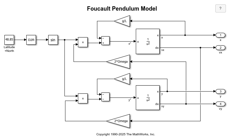
The simplest way to model the Foucault pendulum in Simulink® is to build a model that solves the coupled differential equations for the system. These equations describe the Foucault pendulum system. For details about the derivation of these equations, see Analysis and Physics.


Open the example, which contains the model sldemo_foucault.
mdl='sldemo_foucault';
open_system(mdl);
Initial Conditions
The model loads the constants and initial conditions from the file sldemo_foucault_data.m. The table summarizes the contents of the file. The initial amplitude of the pendulum must be small compared to pendulum length because the differential equations are valid only for small oscillations.
g = 9.83;            % acceleration of gravity (m/s^2)
L = 67;              % pendulum length (m)
initial_x = L/100;   % initial x coordinate (m)
initial_y = 0;       % initial y coordinate (m)
initial_xdot = 0;    % initial x velocity (m/s)
initial_ydot = 0;    % initial y velocity (m/s)
Omega = 2*pi/86400;  % Earth's angular velocity of rotation about its axis (rad/s)
Simulate Foucault Penulum Model
To simulate the model, in the Simulink Toolstrip, on the *Simulate tab, click **Run*. Alternatively, simulate the model programmatically using the sim function.
sldemo_foucault_output = sim(mdl);
The model is configured to run the simulation for 3600 seconds using the stiff variable-step solver ode23t with the default relative tolerance of 1e-6. If you change these settings, the simulation could become numerically unstable over long simulation times. To resolve this issue, use a small enough relative tolerance value and be sure to use a stiff solver.
Visualize and Analyze Simulation Results
The simulation stores the simulation results in the variable sldemo_foucault_output as a Simulink.SimulationOutput object. To plot the simulation results, get the logged output data for the pendulum x- and y- position.
t = sldemo_foucault_output.yout{1}.Values.Time;
x = sldemo_foucault_output.yout{1}.Values.Data;
y = sldemo_foucault_output.yout{3}.Values.Data;
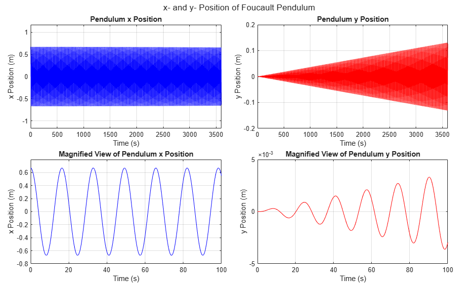
Plot the x- and y- position data using a tiled layout. In the first row, plot the complete x- and y- signals to see how the pendulum position changes over the entire simulation. In the second row, plot a magnified view of the x- and y- data to see a detailed view of how the pendulum position changes within a shorter time range.
figure(1);
tlayout = tiledlayout(2,2);
tlayout.TileSpacing = "compact";
tlayout.Padding = "compact";
title(tlayout,"x- and y- Position of Foucault Pendulum")

nexttile
plot(t,x,Color="b")
axis([0 max(t) min(x) - 0.5 max(x)+0.5])
grid on
title("Pendulum x Position")
xlabel("Time (s)")
ylabel("x Position (m)")

nexttile
plot(t,y,Color="r")
axis([0 max(t) -0.2 0.2])
grid on
title("Pendulum y Position")
xlabel("Time (s)")
ylabel("y Position (m)")

nexttile
plot(t,x,Color="b")
axis([0 100 -0.8 0.8])
grid on
title("Magnified View of Pendulum x Position")
xlabel("Time (s)")
ylabel("x Position (m)")

nexttile
plot(t,y,Color="r")
axis([0 100 -0.005 0.005])
grid on
title("Magnified View of Pendulum y Position")
xlabel("Time (s)")
ylabel("y Position (m)")
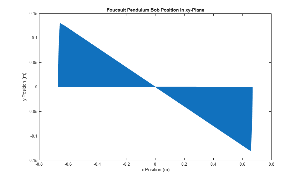
The pendulum oscillation plane takes more than 24 hours to complete a 360 degree sweep. The sweep period is a function of geographic latitude lambda. For details, see the derivation in Analysis and Physics.
To visualize the rotation of the pendulum oscillation plane, plot the y-position data against the x-position data.
figure(2);
plot(x,y)
title("Foucault Pendulum Bob Position in xy-Plane")
xlabel("x Position (m)")
ylabel("y Position (m)")
To animate the visualization of the pendulum oscillation plane rotation, call the script sldemo_foucault_animation by typing the name of the script into the MATLAB command prompt.
Analysis and Physics
This section analyzes the Foucault pendulum and describes the physics behind it. The pendulum can be modeled as a point mass suspended on a wire of length L. The pendulum is located at the geographical latitude lambda. It is convenient to use the reference frames shown in the image. The inertial frame I is relative to the center of the Earth. The non-inertial frame N is relative to an observer on the surface of the. The non-inertial frame accelerates as a result of the axial rotation of the Earth.
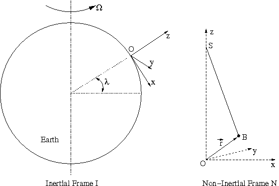
Point O is the origin of the non-inertial frame N. It is the point on the surface of the earth beneath the point of suspension of the pendulum. The non inertial frame is chosen such that the z-axis points away from the center of the Earth and is perpendicular to Earth's surface. The x-axis points south and the y-axis points west.
As mentioned in the introduction, the oscillation plane of a Foucault pendulum rotates. The oscillation plane completes a full rotation in time Trot given by this equation, where Tday is the duration of one day, or the time it takes the Earth to revolve around its axis.

The sine factor requires further discussion. It is often incorrectly assumed that the oscillation plane of the pendulum is fixed in the inertial frame relative to the center of the Earth. This is only true at the north and south poles. To eliminate this confusion, think about the point S, where the pendulum is suspended. In the inertial frame I, point S moves on a circle. The pendulum bob is suspended on a wire of constant length. For simplicity ignore the air friction. In the inertial frame I, there are only two forces that act on the bob - the wire tension T and the gravitational force Fg.
The vector r gives the position of the pendulum bob, B. Newton's second law states that the sum of all forces acting on a body equals the mass times the acceleration of the body.

Throughout this proof, the dots denote time derivatives, arrows denote vectors, caps denote unitary vectors (i, j, and k along x, y, and z axes). A dot above the vector arrow indicated the time derivative of the vector. An arrow above the dot indicated the vector of the time derivative. See the difference between total acceleration and radial acceleration below.
Total Acceleration:

Radial Acceleration:

The acceleration of gravity points towards the center of the earth (negative z-direction).


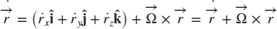
Decompose the acceleration term:


The time derivatives of unit vectors appear because the non-inertial reference frame N is rotating in space. This means that the unitary vectors i, j, and k rotate in space. Their time derivatives are given below. Omega is Earth's angular velocity of revolution around its axis. The scalar Omega is the value of the angular velocity. The vectorial Omega is the vector angular velocity. Its direction is determined by the right hand rule.


Rewrite the time derivative of the vector r relative to Omega.
Similarly, express the second time derivative of the vector r.
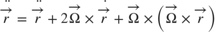

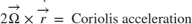

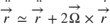
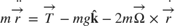
To simplify this equation, assume that Omega for Earth is very small. This allows us to ignore the third term in the equation above. In fact, the second term (which is already much smaller than the first term) is four orders of magnitude greater than the third term. This reduces the equation to the following form:
Newton's Second Law can be written and decomposed into x, y, and z components as follows:


The angular amplitude of oscillations is small. Therefore, we can ignore the vertical velocity and vertical acceleration (z-dot and z-double-dot). The string tension components can be expressed using small angle approximations, which also considerably simplify the problem, making it two-dimensional (see below).


Characteristic Differential Equations
Finally the physics of the problem can be described by the system of coupled equations given below. The x and y coordinates specify the position of the pendulum bob as seen by an observer on Earth.


Analytic Solution (Approximate)
The following is an analytic solution to the Foucault pendulum problem. Unfortunately, it is not exact. If you try to substitute the analytic solution into the differential equations, uncanceled terms of the order Omega squared will remain. However, because Omega is very small, we can ignore the uncanceled terms for practical purposes.


Actual Differential Equation System Is Asymmetric
During the derivation, terms involving Omega squared were ignored. This resulted in xy symmetry in the differential equations. If the Omega squared terms are taken into consideration, the differential equation system becomes asymmetric.


You can easily modify the current Foucault pendulum model to account for asymmetric differential equations. Simply edit the corresponding Gain blocks that contain g/L and add the necessary expression. This change introduces a small overall correction to the numerical result.
See Also
Gain | Second-Order Integrator