Reduced Order Modeler

Create reduced order models based on Simulink models, subsystems within models, or simulation data

Since R2025b

Description

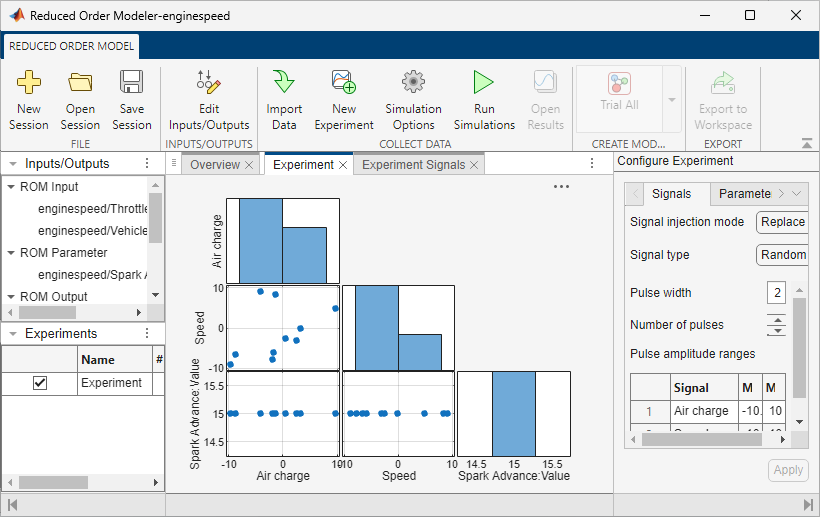
The Reduced Order Modeler app creates AI-based reduced order models (ROMs) of systems modeled in Simulink^®, including full-order, high-fidelity third-party simulation models and subsystems within models. You can also use the app to create ROMs using existing time-domain data. You can use the created ROMs as surrogates for more computationally complex models in applications that require running many simulations.

Using the app, you can:

• Configure experiments to generate input-output training data from a high-fidelity model, or import existing time-domain data for training.

• Train ROMs using pre-configured templates and identify the model that best fits the data.

• Export trained ROMs to Simulink.

After exporting a ROM, you can use it for system-level desktop simulation, control design, hardware-in-the-loop (HIL) testing, virtual sensor modeling, and creation of functional mockup units (FMUs). You can use FMUs outside of MATLAB^® and Simulink.

To install the Reduced Order Modeler for MATLAB Support Package, locate the add-on in Add-On Explorer using the instructions in Get and Manage Add-Ons.

Open the Reduced Order Modeler App

• MATLAB command prompt: Enter reducedOrderModeler.

Examples

• Configure Options in Reduced Order Modeler
• Reduced Order Model of an Airframe (System Identification Toolbox)
• Reduced Order Modeling of Subsystems in Engine Model (System Identification Toolbox)
• Reduced Order Model of a Jet Engine Turbine Blade (System Identification Toolbox)
• Reduced Order Modeling of Battery Electric Vehicle Thermal Management System (System Identification Toolbox)
• Reduced Order Model of a Jet Engine Turbine Blade from Data (System Identification Toolbox)

Programmatic Use

reducedOrderModeler

reducedOrderModeler opens the Reduced Order Modeler dialog box, where you can choose to create a ROM from:

• A Simulink model by entering the file name of a model on the path.

• A MATLAB variable by choosing the variable from the MATLAB workspace.

A new Reduced Order Modeler app session opens for the chosen model or variable.

If you choose a linear time-invariant (LTI) model object as the MATLAB variable, the Model Reducer (Control System Toolbox) app opens.

reducedOrderModeler(modelname)

reducedOrderModeler(modelname) opens the app for the Simulink model modelname. modelname is the name of an open Simulink model or a Simulink model on the path.

reducedOrderModeler(y,u)

reducedOrderModeler(y,u) opens the app along with the Import Data dialog box. This dialog box is prepopulated with inputs and outputs. y and u are matrices that contain uniformly sampled output and input time-domain signal values, respectively. Their dimensions are:

• y — N_s-by-N_y, where N_s is the number of time points and N_y is the number of outputs

• u — N_s-by-N_u, where N_u is the number of inputs

For more information on the Import Data dialog box, see Configure Options in Reduced Order Modeler.

reducedOrderModeler(data)

reducedOrderModeler(data) opens the app along with the Import Data dialog box. This dialog box shows the selected data. data can be:

• An N_s-by-(1+N_u+N_y) matrix or table when you have explicit time data

• An N_s-by-(N_u+N_y) timetable

• An N_s-by-(N_u+N_y) matrix or table when you have no explicit time data

Here:

• N_s is the number of time points.

• N_u is the number of inputs, which can be zero.

• N_y is the number of outputs, which must be at least one.

If data has more columns than rows, the Add Data dialog box opens, where you can choose to import the data by rows or columns. If data does not have more columns than rows, the app directly imports the data by columns.

For more information on the Import Data dialog box, see Configure Options in Reduced Order Modeler.

reducedOrderModeler(sys)

reducedOrderModeler(sys) opens the Model Reducer (Control System Toolbox) app and imports the specified LTI model object, sys. sys can be:

• A tf, ss, or zpk model that is proper. The model can be either single-input single-output (SISO) or multiple-input multiple-output (MIMO), and continuous or discrete.

  • Continuous-time models must not have time delays. To reduce a continuous-time model with time delays, first use pade (Control System Toolbox) to approximate the time delays as model dynamics.

  • Discrete-time models can have time delays. For the Balanced Truncation reduction method, the app uses absorbDelay (Control System Toolbox) to convert the delay into poles at z = 0 before reducing the model. The additional states are reflected in the response plot and Hankel singular-value plot.

• A generalized model such as a genss model. The Model Reducer app uses the current or nominal value of all control design blocks in sys (see getValue (Control System Toolbox)).

• A sparse state-space model such as a sparss or mechss model.

Version History

Introduced in R2025b