Configure Options in Reduced Order Modeler

The Reduced Order Modeler app creates reduced order models (ROMs) of subsystems modeled in Simulink^®, including full-order, high-fidelity third-party simulation models. You can also use the app to create ROMs using existing time-domain data. For information on the app, see Reduced Order Modeler.

To use the Reduced Order Modeler app, you must have the Reduced Order Modeler for MATLAB^® Support Package installed. To install the support package, locate it in Add-On Explorer using the instructions in Get and Manage Add-Ons.

To create ROMs using the app, you need to:

1. Select signals and parameters from the Simulink model as ROM inputs and outputs, or import existing time-domain data.

2. Configure experiments to set up the conditions for simulations.

3. Run simulations of the original model and collect data.

4. Use the data you collect to train models, then choose one to export as the ROM.

Select ROM Inputs and Outputs from Simulink Model

In the Reduced Order Modeler app, you can select Simulink signals or block parameters as ROM inputs and outputs.

To open the app, at the MATLAB command prompt, enter reducedOrderModeler(modelname), where modelname is the name of a Simulink model on the path. You can also enter reducedOrderModeler and, in the Reduced Order Modeler dialog box, enter the model name.

In the app, on the Reduced Order Model tab, click New Session. The Select ROM I/Os dialog box opens.

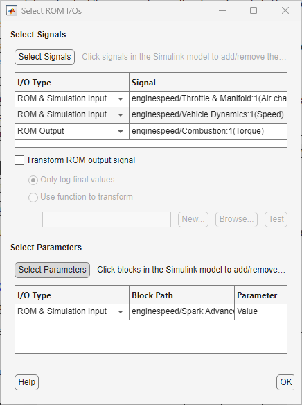
Select Signals

1. To add signals as ROM inputs and outputs, first, click Select Signals. The Simulink model appears in a mode where you can interact with it and select signals. Click the signals you want to add in the Simulink model and select them in the list that appears. The app populates the selected signals in the table below Select Signals in the Select ROM I/Os dialog box.

   To remove selected input and output signals, right-click the signal in the table in the Select ROM I/Os dialog box and click Delete.

2. To set the input or output types of these signals, in the I/O Type column, choose one of these for each signal:

   • ROM Input — ROM input port.

   • ROM Output — ROM output port.

   • Simulation Input — Signal to replace or perturb when you simulate the original model to collect data for training the ROM.

   • ROM & Simulation Input — Both a ROM Input and a Simulation Input. This option is the default type.

   You must set the I/O Type of at least one signal as ROM Output and at least one signal as Simulation Input or ROM & Simulation Input.

3. To alter the signals you set as ROM Output, select the Transform ROM output signal check box.

   • To postprocess logged data and store only the output signal value at the last time point, select Only log final values. Select this option if you want to create a static ROM.

   • To postprocess logged data as defined in a function, select Use function to transform. You can use this option to create both static and dynamic ROMs.

     To specify the function to use, click Browse in the Select ROM I/Os dialog box and select a function, or enter the name of the function in the text box.

     If the function you need is not available, you can define a new function. Click New in the Select ROM I/Os dialog box. The Post Simulation Function Templates dialog box opens. Select a post-simulation function template to use and click OK. Define the function by editing the template in the MATLAB editor. Save the function, and then, in the Select ROM I/Os dialog box, specify it as the function to use.

     To debug the function by calling it with prototypical data, click Test.

   If you specify scalar output signal values by selecting Only log final values or by defining a function that transforms the outputs into scalar values, you must select parameters and set their I/O Type as ROM & Simulation Input. You cannot set the I/O Type of any signal as Simulation Input or ROM & Simulation Input. For an example, see Reduced Order Modeling of Battery Electric Vehicle Thermal Management System (System Identification Toolbox).

Select Parameters

1. To add block parameters as ROM inputs, first, click Select Parameters. The Simulink model appears in a mode where you can interact with it and select parameters. Click the blocks corresponding to the parameters you want to add in the Simulink model, and select the parameters in the list that appears. The app populates the selected block parameters in the table below Select Parameters in the Select ROM I/Os dialog box.

   To remove selected signals, right-click the parameter in the table in the Select ROM I/Os dialog box and click Delete.

2. In the I/O Type column, set the type of each parameter as one of these options:

   • Simulation Input — Signal to replace or perturb when you simulate the original model to collect data for training the ROM

   • ROM & Simulation Input — Both a ROM Input and a Simulation Input. This option is the default type.

The app populates the selected ROM inputs and outputs in the Inputs/Outputs pane. To edit these inputs and outputs, on the Reduced Order Model tab, click Edit Inputs/Outputs. The Select ROM I/Os dialog box opens with the selected inputs and outputs.

Import Time-Domain Data as ROM Inputs and Outputs

In the Reduced Order Modeler app, you can import your own time-domain data as ROM inputs and outputs.

To open the app, enter:

• reducedOrderModeler(y,u), where y and u are matrices that contain uniformly sampled output and input time-domain signal values, respectively. Their dimensions are:

  • y — N_s-by-N_y, where N_s is the number of time points and N_y is the number of outputs

  • u — N_s-by-N_u, where N_u is the number of inputs

• reducedOrderModeler(data), where data is a matrix, table, or timetable. For information on the supported formats for data, see Supported Data Formats.

You can also enter reducedOrderModeler in the command line and, in the Reduced Order Modeler dialog box, choose a variable from the MATLAB workspace.

The app and the Import Data dialog box open. The data you selected appears in the table in the dialog box. To import additional data, including parameters, choose workspace variables from the Data to import menu and click Add. The app adds table rows for the new data.

• The Name column specifies the port names, which must be unique. You can edit the entries in this column.

• The Type column enables you to specify Input, Output, Time, or Parameter. You can only specify Type as Time in one row, and you must specify Type as Output in at least one row. You can set Type as Parameter only if the data in that row is a scalar.

  If you use the syntax reducedOrderModeler(data) to open the app, by default, Type is Input for all rows (except for the row containing time data, if the data is a timetable).

  For timetables, the app automatically sets Type as Time for the row containing the time data.

• The Data column shows how the app extracts data from the workspace variable and assigns it to the corresponding rows. You cannot edit this column.

To delete one or more table rows, select the row(s) and click Delete Row(s).

If you did not set the Type of any row as Time, select the Time is implicit option and specify Sample time as a finite positive integer. Sample time represents the time interval, in seconds, between two consecutive signal values.

To import the table data into the app, click Import.

Selecting ROM inputs and outputs from a Simulink model or importing time-domain data as ROM inputs and outputs fixes the input/output/parameter ports. To import additional data, on the Reduced Order Modeler tab, click Import Data. The Import Data dialog box opens with the Name and Type columns fixed, that is, you cannot change the entries in these columns. You can choose variables from the Data to Import menu and edit the rows in the Data column to match the corresponding ports.

Supported Data Formats

To import existing time-domain data using the reducedOrderModeler(data) syntax, specify data as one of the following:

• N_s-by-(1+N_u+N_y) matrix or table when you have time data

• N_s-by-(N_u+N_y) timetable

• N_s-by-(N_u+N_y) matrix or table when you have no explicit time data

Here:

• N_s is the number of time points.

• N_u is the number of inputs, which can be zero.

• N_y is the number of outputs, which must be at least one.

If data has more columns than rows, an Add Data dialog box opens, where you can choose to import the data by rows or columns. If data does not have more columns than rows, the app directly imports the data by columns.

Configure Experiments

Create experiments to set up the conditions for simulations.

In the app, on the Reduced Order Modeler tab, click New Experiment. The Configure Experiment pane opens in the app. You can configure multiple experiments by clicking New Experiment for each experiment. All experiments appear in the Experiments pane.

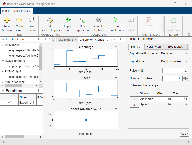
Signals Tab

In the Signal injection mode menu, select one of these modes.

Mode	Description
Replace (Default)	Replace the values of each simulation input signal in the model with the respective generated signal.
Perturb	Add the respective generated signal to the values of each simulation input signal in the model as perturbations.

In the Signal type menu, select one of these types.

Type	Description
Random pulses (Default)	Select pulse amplitudes at random within the range you specify for each simulation input.
Binary sequence	Select the pulses to be a pseudorandom sequence of the maximum or minimum values of each pulse amplitude range.
Sobol sequence	Generate pulses from the quasi-random Sobol sequence within the specified pulse amplitude ranges.
Chirp signal	Generate a chirp signal for each signal with specified initial and final frequencies, initial phase, minimum and maximum amplitudes, and target time.
Custom signal	Specify a custom signal.

If you select the Random pulses, Binary sequence, or Sobol sequence signal type, specify:

• Pulse width — Duration of each pulse in seconds, specified as a positive scalar

• Number of pulses — Number of pulses that the app must generate, specified as a positive integer

• Pulse amplitude ranges

  • Min — Minimum value of the pulse amplitude of the corresponding signal, specified as a scalar (less than Max)

  • Max — Maximum value of the pulse amplitude of the corresponding signal, specified as a scalar (greater than Min)

Additionally, for the Binary sequence signal type, specify:

• Sequence order — Order of the pseudorandom binary sequence pattern, specified as a positive integer

For the Chirp signal signal type, specify:

• Initial frequency (Hz) — Instantaneous frequency of each signal at start time, specified as a vector of nonnegative scalars. The length of the vector is equal to the number of signals. If you specify Initial frequency (Hz) as a scalar, the software automatically creates a vector by assigning the same value to all signals.

• Final frequency (Hz) — Instantaneous frequency of each signal at target time, specified as a vector of nonnegative scalars. The length of the vector is equal to the number of signals. If you specify Final frequency (Hz) as a scalar, the software automatically creates a vector by assigning the same value to all signals.

• Initial phase (deg) — Phase of each signal at start time, specified as a vector. The length of the vector is equal to the number of signals. If you specify Initial phase (deg) as a scalar, the software automatically creates a vector by assigning the same value to all signals.

• Minimum amplitude — Minimum amplitude of each signal, specified as a vector. The length of the vector is equal to the number of signals. If you specify Minimum amplitude as a scalar, the software automatically creates a vector by assigning the same value to all signals.

• Maximum amplitude — Maximum amplitude of each signal, specified as a vector. The length of the vector is equal to the number of signals. If you specify Maximum amplitude as a scalar, the software automatically creates a vector by assigning the same value to all signals.

• Target time (sec) — End time, specified as a positive scalar.

For the Custom signal signal type, specify:

• Custom signal — Timetable or two-column array ([t,u]) for each signal, where t is the time value and u is the signal value

Parameters Tab

In the Method menu, select one of these methods.

Method	Description
Values (Default)	Specify the values of the selected parameters explicitly.
Distribution	Specify the values of the selected parameters in the form of a distribution.

If you select the Values method, specify the value of each selected parameter in the table as a scalar or vector. If you specify a scalar, the parameter adopts only one value. If you specify a vector, the parameter adopts all of the values in the vector. If you select multiple parameters, the app runs a different simulation for each combination of parameter values. In the Experiments pane, # Sims displays the total number of simulations.

If you select the Distribution method, in the Number of samples field, specify the number of samples that the app must generate as a positive integer. To specify the distribution from which the app samples the parameter values, click Edit Distributions. In the Edit Distributions dialog box, choose the sampling method, the parameter probability distributions, and whether the parameters are cross correlated.

For more information, see the Sampling Method and Probability Distribution sections in the topic Generate Random Parameter Values (Simulink Design Optimization).

Boundaries Tab

If you select Random pulses, Binary sequence, or Sobol sequence as the signal type, you can specify boundaries for signal and parameter values to exclude values that are not physically feasible. In the Removal method menu, select one of these methods.

Removal method	Description
Reject and resample (Default)	Reject all signal or parameter values that are not within the specified boundary and repeat the sampling process until you obtain replacements for the rejected values or reach the maximum number of iterations.
Move onto the feasible region	Project each out-of-boundary signal or parameter value onto the specified boundary region.

To specify boundaries for the signal or parameter values, click Edit Boundaries. The Edit Boundaries dialog box opens.

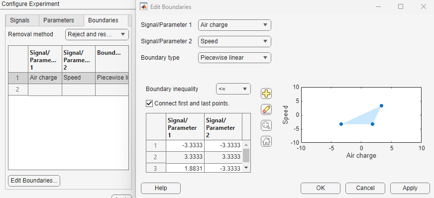
1. In the Signal/Parameter 1 and Signal/Parameter 2 menus, select either a signal or a parameter depending on the pair of signals, parameters, or one of each for which you want to define a boundary.

2. In the Boundary type menu, set the type of boundary as either Piecewise linear or Elliptical. For each pair of signals/parameters, you can define only one type of boundary, either Piecewise linear or Elliptical, but not both.

   1. Piecewise linear — If you select Connect first and last points, you must specify at least three vertices to define the boundary. Otherwise, you must specify at least two vertices. Specify the vertices using one of these methods:

      • To add a vertex to the plot, click the add button and click on the plot in the desired location. To delete a vertex, click the erase button and then click the vertex you want to remove. Click the add and erase buttons again once you are done. To edit the vertices, drag the points on the plot. You can zoom in or out using and reset the level of zoom using .

      • To add or edit a vertex using the table, enter or edit its values in the table.

   2. Elliptical — Edit the Center point and Axes lengths of the boundary using the table. Specify the angle of the boundary using the Rotation (deg) text box. You can zoom in or out using and reset the level of zoom using .

3. In the Boundary inequality menu, select <= or >= to include or exclude the region within the specified boundary, respectively. The included region is shaded.

4. Click OK. On the Boundaries tab, you can see that the table is populated with the specified boundary.

When you define boundary conditions for a pair of signals (or parameters), they cannot conflict with boundaries that you have already defined for either signal (or parameter) as part of another pair. If the boundaries conflict, the app displays an error and does not apply the latest boundary condition.

The app associates the boundary conditions you define with only this experiment. To add boundaries to a new experiment, you must define the boundary conditions again.

To add the specified boundaries to the experiment and visualize their effects, in the Configure Experiments pane, click Apply. The app updates the scatter plot so that the sample points are within the boundaries.

Run Simulations

To run simulations and collect data, on the Reduced Order Model tab, click Simulation Options. The Run Options dialog box opens. Here, you can choose to:

• Log the original Simulink model states.

• Log either all signals in the original model, or just the ROM inputs and outputs.

• Not log untransformed outputs when using a transform output function.

• Log simulation results to a specified file.

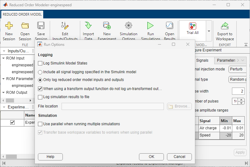
To run simulations in parallel, select Use parallel when running multiple simulations. When you run simulations in parallel, the software transfers all base workspace variables to the workers by default. If your workspace contains variables that you do not want the software to transfer, unselect the Transfer base workspace variables to workers when using parallel option.

After you configure the options, run the simulations. In the app, on the Reduced Order Model tab, click Run Simulations. In the Experiments pane, Results stores the simulation results. The Simulation Result tab opens in the app along with a plot of the results.

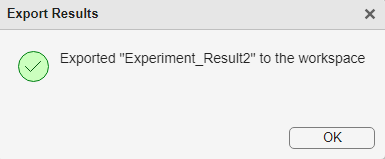
You can export simulation results to the MATLAB workspace. On the Reduced Order Model tab, click Export to Workspace. Click Export to Workspace to open the Export Results dialog box, then select the experiments whose results you want to export, and click OK. In this dialog box, the Simulation Results column shows how many simulation results you are exporting from each experiment. To exclude specific simulation results when exporting an experiment, see Simulation Result Tab.

Simulation Result Tab

To open the results plot of an experiment, select that experiment in the Experiments pane and, on the Reduced Order Model tab, click Open Results.

In the app, on the Simulation Result tab, in the Simulation Results section, you can choose an individual simulation to view its result in the Result tab. In the Options section, if you did not specify a scalar output signal, you can choose whether to show the result as scatter plots, show only the output, or both. In contrast, if you specified a scalar output signal, you can either show the result as a scatter plot, show the output as a distribution, or show any simulation errors.

If you do not want to use the result in view to train the ROM in Experiment Manager, in the Export Result section, clear the When training model option. The app automatically clears and disables this option if the result in view has errors. To exclude the result in view when exporting the results of the experiment to the workspace, clear the When exporting experiment option.

To export only the result in view to the workspace, click Export to Workspace. The Export Results dialog box opens. Click OK.

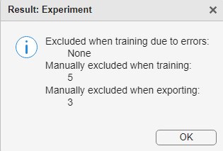
To view which simulation results, if any, the app excluded due to errors or you excluded manually, in the Simulation Results section, click Show Excluded Results.

Train ROM

After you have specified the ROM inputs and outputs, configured experiments, and run simulations of the original model, you can use the simulation results to train models. You can then export a trained model to use as a ROM.

In the app, on the Reduced Order Model tab, in the Create Model section, click the type of model you want to train. The Export Results dialog box opens. In the first table in this dialog box, select experiments to use for training. The Simulation Results column of this table shows how many simulation results you are using from each experiment. To exclude specific simulation results for model training, see Simulation Result Tab.

In the second table, select the ROM input and output signals that you want to use in a model training experiment. If the ROM output signals are not scalar, you must select at least one input and one output signal. If the ROM output signals available in the table have scalar values, you must select at least one output signal. By default, all signals are selected. Click OK. In the Create Experiment dialog box, either choose New Project to create a new experiment project, or choose Existing Project and open an existing experiment project. The Experiment Manager opens.

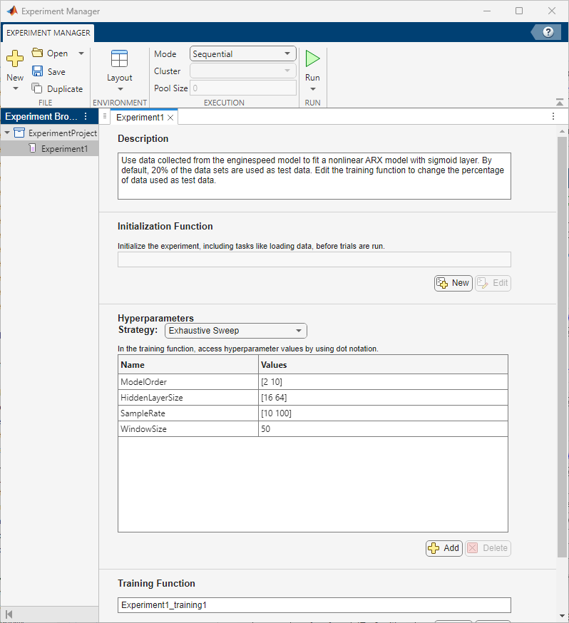
To view experiment information such as the high-fidelity system, ROM model type, and test data percentage in Experiment Manager, view the Description text box.

Specify Training Options

In the Hyperparameters Strategy menu, select one of these methods.

Method	Description
Exhaustive Sweep (Default)	Sweep through a range of hyperparameter values to train models. In the Values column, you specify each hyperparameter value in the form of a scalar or vector.
Bayesian Optimization	Use Bayesian optimization and find optimal training options to train models. In the Range column, you specify a range, in the form of a two-element vector, from which the app takes the hyperparameter values.
Random Sampling	Randomly sample the hyperparameters from a specified probability distribution. In the Distribution menu, select a probability distribution for each hyperparameter and specify the required values in the Values column.

This table shows the hyperparameters whose values you have to specify for each type of model.

Model	Hyperparameter	Description
Nonlinear ARX	SampleRate	Sampling rate of the trained model, specified as a positive scalar
	ModelOrder	Number of poles or the number of states in the model specified as a positive integer
	HiddenLayerSize	Number of neurons in each hidden layer of the network, specified as a positive integer
	WindowSize	Number of samples in each frame or batch when the app segments data for model training, specified as a positive integer
Neural State Space	SampleRate	Sampling rate of the trained model, specified as a positive scalar
	HiddenLayerSize	Number of neurons in each hidden layer of the network, specified as a positive integer
	NumberLayers	Number of layers in the neural network, specified as a positive integer
	NumberInputLags	Delay between the time at which input is received and the time at which it affects the system state, specified as a positive integer
	NumberOutputLags	Additional states that are delays of the original states, specified as a positive integer
	WindowSize	Number of samples in each frame or batch when the app segments data for model training, specified as a positive integer
	Overlap	Number of samples in the overlap between successive frames when the app segments data for model training, specified as an integer
Cascade-Correlation	ModelOrder	Number of poles or the number of states in the model, specified as a positive integer
	SampleRate	Sampling rate of the trained model, specified as a positive scalar
	WindowSize	Number of samples in each frame or batch when the app segments data for model training, specified as a positive integer
	MaxNumActLayer	Maximum number of activation layers in the cascade-correlation neural network, specified as a positive integer
	CrossValidate	Option to reserve data for cross-validation, specified as "true" or "false"
	HoldoutFraction	Fraction of training data used for cross-validation, specified as a positive scalar less than or equal to 1
LSTM Network	SampleRate	Sampling rate of the trained model, specified as a positive scalar
	HiddenLayerSize	Number of neurons in each hidden layer of the network, specified as a positive integer
	NumberLayers	Number of layers in the neural network, specified as a positive integer
	InitialLearnRate	Initial learning rate used for training, specified as a positive scalar
MLP Network	HiddenLayerSize	Number of neurons in each hidden layer of the network, specified as a positive integer
	NumberLayers	Number of layers in the neural network, specified as a positive integer
Gridded Interpolant (For static ROMs only)	Method	Interpolation method, specified as a string or string array containing ["linear","nearest","next","previous","pchip","cubic","spline","makima"]
	ExtrapolationMethod	Extrapolation method, specified as a string or string array containing ["linear","nearest","next","previous","pchip","cubic","spline","makima","none"]
Scattered Interpolant (For static ROMs only)	Method	Interpolation method, specified as a string or string array containing ["linear","nearest","natural"]
	ExtrapolationMethod	Extrapolation method, specified as a string or string array containing ["linear","nearest","boundary","none"]
Trial All	ModelType	Types of models to create, specified as a string or string array containing ["Cascade-Correlation","Nonlinear ARX","Neural State Space","MLP Network","LSTM Network"]

To create a Gridded Interpolant model, you must select at least two parameters, configure at least one experiment in the Reduced Order Modeler app where you select the Method as Values, and specify at least two values for each parameter. To create a Scattered Interpolant model, you must have a total of at least three simulation results that are included for model training, when you combine all experiments you configured in the Reduced Order Modeler app.

To train all types of models specified in the hyperparameter ModelType, select Trial All as the model type. This training can indicate which model structure produces models with the lowest error values. You can then choose this model structure from the Create Model section, vary the hyperparameters for that model, and train it.

In the Experiment Manager, you can add, delete, and modify hyperparameter values, initialize the experiment in the Initialization Function field, and edit the default Training Function. Additionally, when you select the Bayesian Optimization method, you can customize the Bayesian Optimization Options and Metrics, and when you select the Random Sampling method, you can customize the Random Sampling Options.

On the Experiment Manager tab, in the Mode menu, select the mode in which to run the experiment as Sequential, Simultaneous, Batch Sequential, or Batch Simultaneous. Select the Cluster and Pool Size if you are running the experiment using parallel computing. Click Run.

View and Export Results

The Experiment Manager uses the simulation result data to train a model of the selected type for each of the specified hyperparameter combinations. The last two columns in the results table show the Information and Metrics for each combination. For all model types, the information properties are TrainingMSE (mean squared error calculated on the training data set) and TestMSE (mean squared error calculated on the test data set). The loss metric is TrainingLoss (measure of inaccuracy on the training data set).

On the Experiment Manager tab, in the Review Results section, you can select and visualize different plots for the selected trial.

• Training Plot — Displays the training loss for each iteration.

• Test Data: Actual vs Predicted — Displays a plot of the actual output versus the predicted output for each model output.

• Test Data: Predicted Response — Displays the actual and predicted responses for each model output for time-domain (dynamic) models.

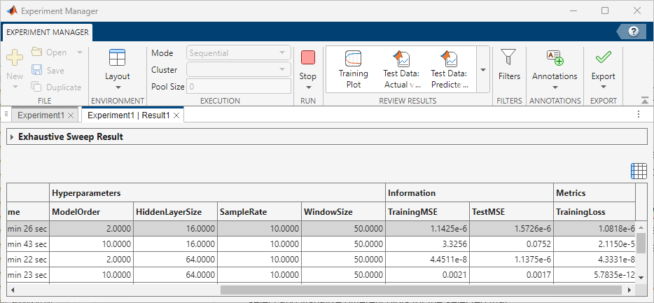
To export the model that best fits the data to the workspace, select the trial with low TestMSE, reasonable TrainingMSE, and low TrainingLoss. On the Experiment Manager tab, click Export and then click Training Output.