Perform Forward and Inverse Kinematics on a Five-Bar Robot
This example shows how to use the KinematicsSolver object to perform forward kinematics (FK) and inverse kinematics (IK) on a five-bar robotic mechanism. First, the example demonstrates how to perform FK analyses to calculate a singularity-free workspace for a five-bar robot. Then the example shows how to perform IK analyses to compute the motor angles that correspond to an end-effector trajectory within that workspace.
A five-bar robot, which is also called a five-bar planar manipulator, is a two-degree-of-freedom parallel mechanism. In this example, the robot has four equal-length links that cannot collide with each other. The robot uses two stepper motors to drive the proximal links to move the pen.

The five-bar robot has four configuration space regimes: --, -+, ++, and +-. As shown in the image, each sign indicates the sign of the offset angle between the corresponding proximal and distal links. The active revolute joints a and b are directly controlled by the motors, and the passive revolute joints c and d connect the proximal and distal links.
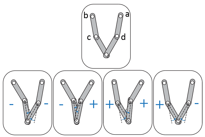
Configurations in which one or both of the arms become fully extended cause the end effector to lose at least one of its degrees of freedom. These configurations correspond to kinematic singularities and occur when the robot transitions from one regime to another. To avoid the kinematic singularities in the FK analysis, this example only studies the five-bar robot workspace in the +- regime.
Run Forward Kinematics on the Five-Bar Robot
This section demonstrates how to perform an FK analysis to compute a singularity-free workspace for the pen that corresponds to a set of motor angles. Specifically, the example assigns the active joint angles of the robot as target variables and the x and y coordinates of the pen as output variables. The example also assigns the passive joints as initial guess variables, which are used to help bias the solutions towards the +- regime.
1. To perform the FK analysis, first load the five-bar robot model into memory and create a KinematicsSolver object (fk) for the model.
mdl = "FiveBar";
load_system(mdl);
fk = simscape.multibody.KinematicsSolver(mdl);
2. To specify and study the relationships between the pen, world frame, active joints, and passive joints of the robot, you need to create frame variables that correspond to the position of the pen with respect to the world frame. Note that you don't need to create joint variables because they are created automatically when the object is constructed.
Add a group of three translational frame variables for the pen to fk. Specify the world frame as the base and the Tip frame of the pen as the follower. Name the frame variable group Pen.
base = mdl + "/World Frame/W";
follower = mdl + "/Five Bar Robot/Pen/Pen/Tip";
addFrameVariables(fk,"Pen","Translation", base, follower);
3. Assign the position-based joint variables of the active joints (j5.Rz.q and j4.Rz.q) as targets. To find the IDs of the position-based joint variables, use the jointPositionVariables object function.
jointPositionVariables(fk)
ans=5×4 table
       ID           JointType                             BlockPath                          Unit
    _________    ________________    ____________________________________________________    _____

    "j1.Rz.q"    "Revolute Joint"    "FiveBar/Five Bar Robot/Passive_Joint_c"                "deg"
    "j2.Rz.q"    "Revolute Joint"    "FiveBar/Five Bar Robot/Passive_Joint_d"                "deg"
    "j3.Rz.q"    "Revolute Joint"    "FiveBar/Five Bar Robot/Passive_Joint_e"                "deg"
    "j4.Rz.q"    "Revolute Joint"    "FiveBar/Five Bar Robot/Step_Motor_a/Active_Joint_a"    "deg"
    "j5.Rz.q"    "Revolute Joint"    "FiveBar/Five Bar Robot/Step_Motor_b/Active_Joint_b"    "deg"
targetIDs = ["j5.Rz.q";"j4.Rz.q"];
addTargetVariables(fk,targetIDs);
4. Assign these variables as outputs:
The translational x and y components of the pen (
Pen.Translation.xandPen.Translation.y)The joint variables of the passive joints (
j1.Rz.qandj2.Rz.q)
To find the IDs of the frame variables, use the frameVariables object function.
frameVariables(fk)
ans=3×4 table
            ID                      Base                            Follower                  Unit
    ___________________    _______________________    ____________________________________    ____

    "Pen.Translation.x"    "FiveBar/World Frame/W"    "FiveBar/Five Bar Robot/Pen/Pen/Tip"    "m"
    "Pen.Translation.y"    "FiveBar/World Frame/W"    "FiveBar/Five Bar Robot/Pen/Pen/Tip"    "m"
    "Pen.Translation.z"    "FiveBar/World Frame/W"    "FiveBar/Five Bar Robot/Pen/Pen/Tip"    "m"
outputIDs = ["Pen.Translation.x";"Pen.Translation.y";"j1.Rz.q";"j2.Rz.q"];
addOutputVariables(fk,outputIDs);
5. Assign the joint variables of the passive joints (j1.Rz.q and j2.Rz.q) as guesses.
guessIDs = ["j1.Rz.q";"j2.Rz.q"];
addInitialGuessVariables(fk,guessIDs);
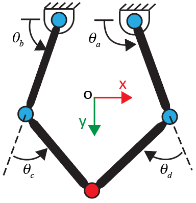
6. The image is a sketch of the five-bar robot. The angles of the active joints are and , and the passive joints are and . Use a nested for loop to compute the workspace of the pen for a set of active joint angles that vary between [95, 150] and [30, 85] degrees, respectively. To ensure that the robot is in the +- regime, use [50 -50] degrees as the initial values for the guess variables (j1.Rz.q and j2.Rz.q) and then use the latest values of the guess variables to guide the next FK solution.
guesses = [50 -50]; % Initial guesses for theta_c and theta_d
index = 1;

% Generate angles for theta_a and theta_b
theta_a = linspace(95,150,31);
theta_b = linspace(30,85,31);

% Allocate memory for output data
ik_data = zeros(length(theta_a)*length(theta_b),length(outputIDs));

% Calculate the robot's workspace for the given theta_a and theta_b
for i = 1:length(theta_a)
    for j = 1:length(theta_b)
        targets = [theta_b(j),theta_a(i)];
        [outputVec,statusFlag] = solve(fk,targets,guesses);
        if statusFlag == 1 % Save a solution if its statusFlag is 1
            ik_data(index,1:length(outputIDs)) = outputVec;
            index = index + 1;
            guesses = [outputVec(3),outputVec(4)]; % Update next guess with last solution
        end
    end
end
7. Plot the angles of the passive joints to verify if the five-bar robot is in the +- regime. If the robot is in the +- regime, the values of and are consistently positive and negative, respectively.
figure
plot(ik_data(1:index-1,3),"b","LineWidth",2); % Note that the total number of the solutions that satisfy statusFlag equals to index-1;
hold on
plot(ik_data(1:index-1,4),"k","LineWidth",2);
hold off


title("Passive Joint Angles")
xlabel("Index")
ylabel("Angle (Degrees)")
legend("Joint c","Joint d")
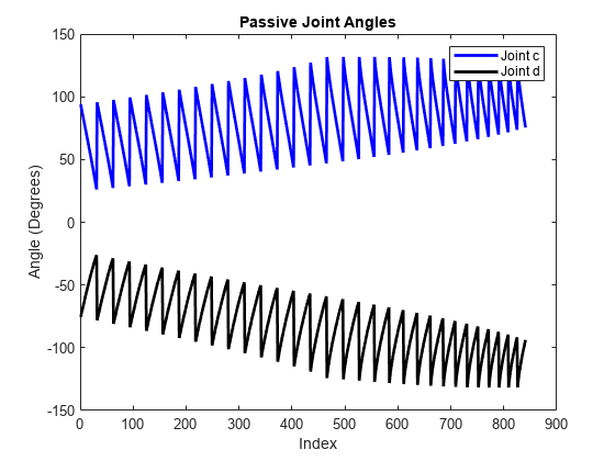
The plot shows that the five-bar robot is in the +- regime. Moreover, the computed workspace is singularity-free because the values of and are away from zero.
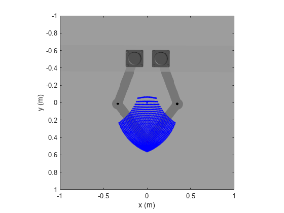
8. Plot the workspace data on the image of the five-bar robot.
% Plot the image of the five-bar robot
figure
x = [-1 1];
y = [1 -1];
C = imread("TopViewFiveBarRobot.png");
image(x,y,C)

hold on

% Plot the calculated workspace as blue dots
plot(ik_data(:,1),ik_data(:,2),"b.")
ylabel("y (m)")
xlabel("x (m)")
axis equal
axis([-1 1 -1 1]);
hold off
Run Inverse Kinematics on the Five-Bar Robot
In this section, the example shows how to perform an IK analysis to compute the motor angles that correspond to an end-effector trajectory. Specifically, the example assigns the translational x and y components of the pen as target variables and assigns the motor angles as output variables. Then the example computes the motor angles for a trajectory of the pen. To ensure the robot is in the +- regime, use the active and passive joint angles as guesses to bias the IK solutions. Note that you need to run the FK section before running this section.
1. Define a circular end-effector trajectory within the previously calculated workspace. Save the coordinates of the circle for the IK analyses.
figure
% Plot the calculated workspace as blue dots on the image of the five-bar robot
image(x,y,C)
hold on
plot(ik_data(:,1),ik_data(:,2),"b.")

% Specify the center and radius of the circle
center_x = 0; % m
center_y = 0.3; % m
radius = 0.15; % m
th = 0:pi/50:2*pi; % radians

% Save the x and y coordinates of the circle for the IK analyses
coordinates_x = radius * cos(th) + center_x;
coordinates_y = radius * sin(th) + center_y;

% Plot the circle
plot(coordinates_x,coordinates_y,"r","LineWidth",2)
axis equal
axis([-1 1 -1 1]);
ylabel("Length (m)")
xlabel("Width (m)")
hold off

2. To perform the IK analysis, first create a KinematicsSolver object (ik) for the model.
ik = simscape.multibody.KinematicsSolver(mdl);
3. Create frame variables for the position of the pen with respect to the world frame and add them to the object (ik). You can reuse the base and follower variables from the FK section.
addFrameVariables(ik, "Pen","Translation", base, follower);
4. Assign the variables that correspond to the translational x and y components of the pen (Pen.Translation.x and Pen.Translation.y) as targets. To find the IDs of the frame variables, use the frameVariables object function.
frameVariables(ik)
ans=3×4 table
            ID                      Base                            Follower                  Unit
    ___________________    _______________________    ____________________________________    ____

    "Pen.Translation.x"    "FiveBar/World Frame/W"    "FiveBar/Five Bar Robot/Pen/Pen/Tip"    "m"
    "Pen.Translation.y"    "FiveBar/World Frame/W"    "FiveBar/Five Bar Robot/Pen/Pen/Tip"    "m"
    "Pen.Translation.z"    "FiveBar/World Frame/W"    "FiveBar/Five Bar Robot/Pen/Pen/Tip"    "m"
targetIds = ["Pen.Translation.x";"Pen.Translation.y"];
addTargetVariables(ik,targetIds);
5. Assign these variables as outputs:
The position-based joint variables of the active joints (
j5.Rz.qandj4.Rz.q)The position-based joint variables of the passive joints (
j1.Rz.qandj2.Rz.q)
To find the IDs of the position-based joint variables, use the jointPositionVariables object function.
jointPositionVariables(ik)
ans=5×4 table
       ID           JointType                             BlockPath                          Unit
    _________    ________________    ____________________________________________________    _____

    "j1.Rz.q"    "Revolute Joint"    "FiveBar/Five Bar Robot/Passive_Joint_c"                "deg"
    "j2.Rz.q"    "Revolute Joint"    "FiveBar/Five Bar Robot/Passive_Joint_d"                "deg"
    "j3.Rz.q"    "Revolute Joint"    "FiveBar/Five Bar Robot/Passive_Joint_e"                "deg"
    "j4.Rz.q"    "Revolute Joint"    "FiveBar/Five Bar Robot/Step_Motor_a/Active_Joint_a"    "deg"
    "j5.Rz.q"    "Revolute Joint"    "FiveBar/Five Bar Robot/Step_Motor_b/Active_Joint_b"    "deg"
outputIds = ["j5.Rz.q";"j4.Rz.q";"j1.Rz.q";"j2.Rz.q"];
addOutputVariables(ik,outputIds);
6. Use a for loop to implement the IK analysis. Specifically, use the for loop to assign the coordinates of the predefined trajectory to the pen and calculate the corresponding motor angles.
N = length(coordinates_x); % Number of points on trajectory
index_in_ik = 1;
ik_data = zeros(N,length(outputIds)); % Allocate memory for the variable

for ind = 1:N
    targets = [coordinates_x(ind), coordinates_y(ind)]; % Use the x and y coordinates of the predefined circle for the inverse kinematics problem
    [outputVec_ik,statusFlag_ik] = solve(ik,targets);
    if statusFlag_ik == 1
        ik_data(index_in_ik,1:length(outputIds)) = outputVec_ik; % save the output data
        index_in_ik = index_in_ik+1;
    else
        error("Did not hit targets");
    end
end
closeViewer(ik);
7. Plot the passive joints of the robot to see if the robot is in the +- regime.
% Plot the angles of the passive joints
figure
plot(ik_data(:,3),"b","LineWidth",2);
hold on
plot(ik_data(:,4),"k","LineWidth",2);
hold off
title("Passive Joint Angles")
xlabel("Point")
ylabel("Angle (Degrees)")
legend("Joint c","Joint d")
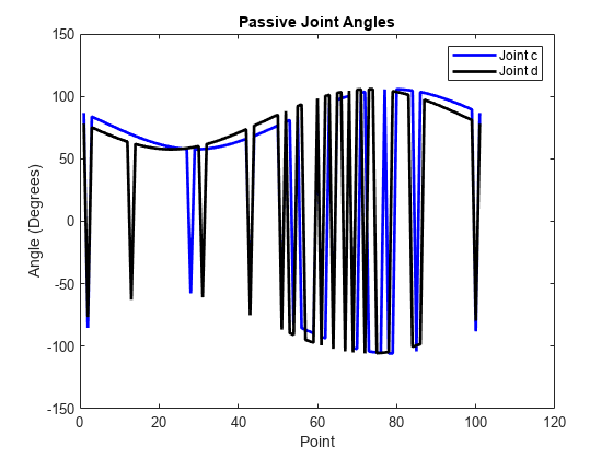
The plot shows that the robot is not always in the +- regime.
8. To help ensure that all solutions stay in the +- regime, assign the joint variables of the passive (j1.Rz.q and j2.Rz.q) and active (j5.Rz.q and j4.Rz.q) joints as guesses to bias the IK solutions.
guessIds = ["j1.Rz.q";"j2.Rz.q";"j5.Rz.q";"j4.Rz.q"];
addInitialGuessVariables(ik,guessIds);
Use [50 -50 45 135] degrees as initial values for the guess variables and use the latest values of the guess variables to guide the next IK solution.
guesses = [50 -50 45 135]; % Assign initial guesses for passive and active joints
N = length(coordinates_x);
index_in_ik = 1;
ik_data = zeros(N,length(outputIds)); % Allocate memory for the variable
for ind = 1:N
    targets = [coordinates_x(ind), coordinates_y(ind)]; % Use the x and y coordinates of the prescribed circle for the inverse kinematics problem
    [outputVec_ik,statusFlag_ik] = solve(ik,targets, guesses);
    if statusFlag_ik == 1
        ik_data(index_in_ik,1:length(outputIds)) = outputVec_ik; % Save the rotations of the motors
        index_in_ik=index_in_ik+1;
        guesses = [outputVec_ik(3) outputVec_ik(4) outputVec_ik(1) outputVec_ik(2)]; % Update next guess with last solution
    else
        error("Did not hit targets");
    end
end
closeViewer(ik);
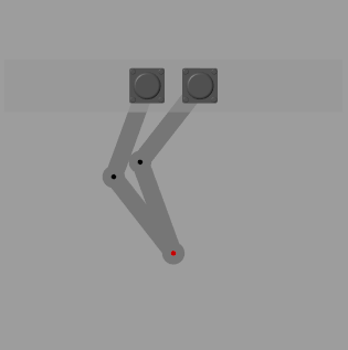
The plot indicates that the passive joint angles are always well away from zero and are always in the +- regime. Therefore, this set of motor angles corresponds to the end effector moving in a smooth motion along the circular trajectory without passing through any kinematic singularities.
% Plot the angles of the passive joints
figure
plot(ik_data(:,3),"b","LineWidth",2);
hold on
plot(ik_data(:,4),"k","LineWidth",2);
hold off
title("Passive Joint Angles")
xlabel("Index")
ylabel("Angle (Degrees)")
legend("Joint c","Joint d")
See Also
KinematicsSolver | frameVariables | initialGuessVariables | jointPositionVariables | outputVariables | targetVariables | addFrameVariables | addInitialGuessVariables | addOutputVariables | addTargetVariables | solve | viewSolution | closeViewer