Heating of Finite Slab

Open Live Script

This example shows how to find the temperature distribution of a one-dimensional finite slab by solving the governing differential equation. The example uses Symbolic Math Toolbox™ to solve the problem of heat transfer analytically in a finite slab as discussed in [1].

The finite slab has constant thermal properties. Assume that heat transfer is due only to conduction with a given thermal diffusivity $α = \frac{k}{ρ c_{p}}$ . The slab is located in the space between $y = - b$ and $y = b$ , where heat propagates along the $y$ -direction. Initially, the slab is at temperature $T_{0}$ . At time $t = 0$ , the edges at $y = \pm b$ are suddenly raised to temperature $T_{1}$ and maintained there. This example solves for the temperature distribution of the slab $T (y, t)$ as a function of the $y$ -coordinate and time $t$ by following these steps:

Define the heat transfer equation.
Use the method of separation of variables.
Apply boundary conditions to find the mode solutions.
Find the coefficients of the general solution by computing the integral of orthogonal functions.
Plot the solution for the temperature as a function of the $y$ -coordinate and time.

One-dimensional slab with a thermal diffusivity alpha and initial temperature T0 at t = 0. Both the left and right edges of the slab at y = -b and y = b is set at a temperature T1 at t > 0.

Define Heat Transfer Equation

For a three-dimensional homogeneous medium, the heat transfer equation due to conduction is given by

$\frac{\partial T}{\partial t} = α (\frac{\partial^{2} T}{\partial x^{2}} + \frac{\partial^{2} T}{\partial y^{2}} + \frac{\partial^{2} T}{\partial z^{2}})$ .

Because heat is transferred along the $y$ -direction, you can reduce the heat transfer equation to

$\frac{\partial T}{\partial t} = α \frac{\partial^{2} T}{\partial y^{2}}$ .

Next, define these dimensionless variables:

Dimensionless temperature $Θ = \frac{T_{1} - T}{T_{1} - T_{0}}$
Dimensionless coordinate $η = \frac{y}{b}$
Dimensionless time $τ = \frac{α t}{b^{2}}$

The differential equation for the heat transfer in terms of these dimensionless variables is

$\frac{\partial Θ}{\partial τ} = \frac{\partial^{2} Θ}{\partial η^{2}}$ ,

where the initial condition at $τ = 0$ is $Θ = 1$ , and the boundary conditions at $η = \pm 1$ are $Θ = 0$ for $τ > 0$ .

Define the main differential equation.

syms Theta(eta,tau)
eqMain = diff(Theta,tau) == diff(Theta,eta,eta)

eqMain(eta, tau) = 
 $\frac{\partial}{\partial τ} Θ (η, τ) = \frac{\partial^{2}}{\partial η^{2}} Θ (η, τ)$

Method of Separation of Variables

Use the method of separation of variables to find the solution for $Θ (η, τ)$ . This method separates the spatial and time dependencies by writing them as a product of spatial and time-dependent functions, where $Θ (η, τ) = f (η) g (τ)$ .

syms f(eta) g(tau)
eqTheta = Theta(eta,tau) == f(eta)*g(tau)

eqTheta =  $Θ (η, τ) = f (η) g (τ)$

Substitute this ansatz into the differential equation.

eqMain = subs(eqMain,lhs(eqTheta),rhs(eqTheta))

eqMain(eta, tau) = 
 $f (η) \frac{\partial}{\partial τ} g (τ) = g (τ) \frac{\partial^{2}}{\partial η^{2}} f (η)$

Separate the $f$ and $g$ terms so that they are be on different sides of the equation.

eqMain = eqMain/g(tau)/f(eta)

eqMain(eta, tau) = 
 $\frac{\frac{\partial}{\partial τ} g (τ)}{g (τ)} = \frac{\frac{\partial^{2}}{\partial η^{2}} f (η)}{f (η)}$

Set each side of the equation to a constant. For convenience, let this constant be $- c^{2}$ .

syms c real
eq1(tau) = lhs(eqMain) == -c^2

eq1(tau) = 
 $\frac{\frac{\partial}{\partial τ} g (τ)}{g (τ)} = - c^{2}$

eq2(eta) = rhs(eqMain) == -c^2

eq2(eta) = 
 $\frac{\frac{\partial^{2}}{\partial η^{2}} f (η)}{f (η)} = - c^{2}$

Apply Boundary Conditions to Find Mode Solution

Next, find the solutions for $f (η)$ and $g (τ)$ by applying the appropriate boundary conditions.

Solve the first-order differential equation for $g (τ)$ by using dsolve.

gsol(tau) = dsolve(eq1)

gsol(tau) =  $C_{1} e^{- c^{2} τ}$

For $f (η)$ , find the even solution based on the symmetry along the $y$ -axis. Because the slab is located at $- b$ to $b$ and the temperature at both edges is fixed at $T_{1}$ , the function $f (η)$ is symmetrical with respect to the origin. Find the general solution using dsolve.

fsol(eta) = dsolve(eq2)

fsol(eta) =  $C_{1} \cos (c η) - C_{2} \sin (c η)$

For a well-behaved function, you can also write the general solution as $f (η) = f_{e v e n} (η) + f_{o d d} (η)$ . The even part of this solution is $f_{e v e n} (η) = \frac{f (η) + f (- η)}{2}$ and the odd part of this solution is $f_{o d d} (η) = \frac{f (η) - f (- η)}{2}$ . Define the even solution of $f (η)$ .

fsol_even(eta) = (fsol(eta) + fsol(-eta))/2

fsol_even(eta) =  $C_{1} \cos (c η)$

Symbolic Math Toolbox uses $C_{1}$ as a dummy variable to represent a constant. In the solutions for $f (η)$ and $g (τ)$ above, the variable $C_{1}$ represents different constants. Rewrite the variable $C_{1}$ from the even solution of $f (η)$ as $C_{f}$ .

syms C1 C_f
fsol = subs(fsol_even,C1,C_f)

fsol(eta) =  $C_{f} \cos (c η)$

Apply the other boundary condition at $η = \pm 1$ , where $f (1) = 0$ , and solve for the parameter $c$ .

[csol,params,conds] = solve(fsol(1)==0,c,ReturnConditions=true)

csol = 
 $\frac{π}{2} + π k$

params =  $k$

conds =  $k \in Z \land C_{f} \neq 0$

The parameter $c$ in the solutions for $f (η)$ and $g (τ)$ depends on an integer parameter $k$ , where $c = π / 2 + π k$ .

Substitute the solutions for $f (η)$ and $g (τ)$ into $Θ (η, τ)$ .

eqTheta = subs(eqTheta,{f g},{fsol gsol})

eqTheta =  $Θ (η, τ) = C_{1} C_{f} e^{- c^{2} τ} \cos (c η)$

Rewrite the $C_{1} C_{f}$ constant term as $C_{k}$ . Rewrite the solution to depend on $k$ as well. This mode solution uses the index $k$ for the dimensionless temperature $Θ (η, τ)$ .

syms C(k) D(k)
eqTheta = subs(eqTheta,{C1*C_f c},{C(k) csol})

eqTheta = 
 $Θ (η, τ) = \cos (η (\frac{π}{2} + π k)) e^{- τ {(\frac{π}{2} + π k)}^{2}} C (k)$

Compute Integral of Orthogonal Functions

Next, construct the general solution of the differential equation from the mode solution. Get the right side of the equation in eqTheta to perform further computations.

Theta_k(eta,tau,k) = rhs(eqTheta)

Theta_k(eta, tau, k) = 
 $\cos (η (\frac{π}{2} + π k)) e^{- τ {(\frac{π}{2} + π k)}^{2}} C (k)$

Following the steps in the textbook [1], combine the terms with indices $k$ and $- (k + 1)$ . Simplify these combined terms.

Theta_k2(eta,tau,k) = simplify(Theta_k(eta,tau,k) + Theta_k(eta,tau,-(k+1)))

Theta_k2(eta, tau, k) = 
 $e^{- \frac{τ π^{2} {(2 k + 1)}^{2}}{4}} \cos (\frac{π η (2 k + 1)}{2}) (C (- k - 1) + C (k))$

Rewrite the general solution by summing all of these modes. Here, define another $D (k)$ coefficient to represent $C (- k - 1) + C (k)$ . Then, take the summation of the $k$ indices from 0 to $\infty$ .

Theta_sol = symsum(subs(Theta_k2,C(-k-1)+C(k),D(k)),k,0,Inf)

Theta_sol(eta, tau) = 
 $\sum_{k = 0}^{\infty} e^{- \frac{τ π^{2} {(2 k + 1)}^{2}}{4}} \cos (\frac{π η (2 k + 1)}{2}) D (k)$

Next, find the $D (k)$ coefficient based on the initial condition of the problem. To do this, set the boundary condition and find the integral of the orthogonal functions that involve the $\cos$ function. Set the initial boundary condition $Θ (η, 0) = 1$ .

ThetaBound = Theta_sol(eta,0) == 1

ThetaBound = 
 $\sum_{k = 0}^{\infty} \cos (\frac{π η (2 k + 1)}{2}) D (k) = 1$

Multiply both sides of the above equation by $\cos (π η (m + \frac{1}{2}))$ , and find the integral with respect to $d η$ . Here, the indices $m$ and $k$ are integers.

syms m k integer
ThetaBound = ThetaBound*cos((m+1/2)*pi*eta)

ThetaBound = 
 $\cos (π η (m + \frac{1}{2})) (\sum_{k = 0}^{\infty} \cos (\frac{π η (2 k + 1)}{2}) D (k)) = \cos (π η (m + \frac{1}{2}))$

ThetaBound = int(lhs(ThetaBound),eta,-1,1) == int(rhs(ThetaBound),eta,-1,1)

ThetaBound = 
 $\int_{- 1}^{1} \cos (π η (m + \frac{1}{2})) (\sum_{k = 0}^{\infty} \cos (\frac{π η (2 k + 1)}{2}) D (k)) d η = \frac{2 \sin (π (m + \frac{1}{2}))}{π (m + \frac{1}{2})}$

This integration involves a symbolic summation series that uses the symsum function. Symbolic Math Toolbox does not find this integral explicitly, so you need to investigate the integral of each summation term on the left side of the above equation. Extract each symbolic summation term that has the indices $m$ and $k$ . Define this term as a new expression. You can copy and paste from the output above when defining this expression manually.

expr_temp = cos(sym(pi)*eta*(m + sym(1/2)))*cos((sym(pi)*eta*(2*k + 1))/2)*D(k)

expr_temp = 
 $\cos (π η (m + \frac{1}{2})) \cos (\frac{π η (2 k + 1)}{2}) D (k)$

Next, find the integral of the expression over $η$ from $- 1$ to $1$ .

expr_int = int(expr_temp,eta,-1,1)

expr_int = 
 ${\begin{array}{cl} D (k) & if k = m \lor k + m = - 1 \\ 0 & if k \neq m \land k + m \neq - 1 \end{array}$

Symbolic Math Toolbox simplifies the integral. To compare this result with the one in the textbook without simplification, check this integral by assuming that $m$ and $k$ are equal (as in the first piecewise condition above).

expr_temp2 = cos(pi*eta*(m+1/2))*cos(pi*eta*(m+1/2))*D(m)

expr_temp2 = 
 ${\cos (π η (m + \frac{1}{2}))}^{2} D (m)$

Without simplification, Symbolic Math Toolbox returns the integral as in the textbook example.

expr_int2 = int(expr_temp2,eta,-1,1)

expr_int2 = 
 $D (m) (\frac{\sin (2 π (m + \frac{1}{2}))}{2 π (m + \frac{1}{2})} + 1)$

Because $m$ is an integer, you can simplify this result.

expr_int2 = simplify(expr_int2)

expr_int2 =  $D (m)$

Next, find the coefficient $D (m)$ by applying the boundary condition from the previous step. Simplify the equation for $D (m)$ with the applied boundary condition, and isolate $D (m)$ on the left side of the equation.

ThetaBound = expr_int2 == rhs(ThetaBound)

ThetaBound = 
 $D (m) = \frac{2 \sin (π (m + \frac{1}{2}))}{π (m + \frac{1}{2})}$

ThetaBound = isolate(simplify(ThetaBound),D(m))

ThetaBound = 
 $D (m) = \frac{4 {(- 1)}^{m}}{π + 2 π m}$

Change the dummy variable $m$ to $k$ . Finally, substitute $D (k)$ into the general solution. This solution represents the heat transfer of a finite one-dimensional slab.

ThetaBound = subs(ThetaBound,m,k);
Theta_sol = subs(Theta_sol,D,rhs(ThetaBound))

Theta_sol(eta, tau) = 
 $4 (\sum_{k = 0}^{\infty} \frac{{(- 1)}^{k} e^{- \frac{τ π^{2} {(2 k + 1)}^{2}}{4}} \cos (\frac{π η (2 k + 1)}{2})}{π + 2 π k})$

Plot Solution for Temperature

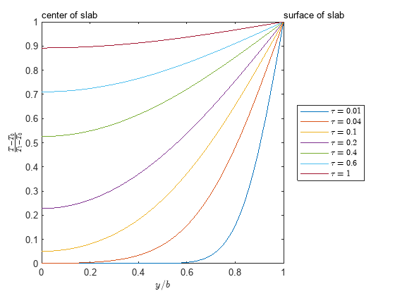
Plot the dimensionless temperature of the slab as a function of $η$ at various values of $τ$ . Because the temperature solution involves a summation series with infinite terms, evaluating all these terms when plotting can be slow. To improve the plotting performance, you can approximate the infinite summation series as a summation series of up to $k = 40$ . Note that the temperature solution is a converging series and numerically stable. For this reason, approximating the series works well to improve the plotting performance.

Theta_sol_approx = subs(Theta_sol,Inf,40);

Plot the temperature of the slab for various values of $τ$ by using fplot.

% Plot the result as in figure 12.1-1 of reference [1]
fplot(eta,1-Theta_sol_approx(eta,0.01),[0 1])
axis equal
hold on
fplot(eta,1-Theta_sol_approx(eta,0.04),[0 1])
fplot(eta,1-Theta_sol_approx(eta,0.1),[0 1])
fplot(eta,1-Theta_sol_approx(eta,0.2),[0 1])
fplot(eta,1-Theta_sol_approx(eta,0.4),[0 1])
fplot(eta,1-Theta_sol_approx(eta,0.6),[0 1])
fplot(eta,1-Theta_sol_approx(eta,1),[0 1])

text(0,1.03,"center of slab")
text(1,1.03,"surface of slab")
xlabel("$y/b$",interpreter="latex")
ylabel("$\frac{T-T_0}{T_1-T_0}$",interpreter="latex")

legend("$\tau=0.01$","$\tau=0.04$","$\tau=0.1$","$\tau=0.2$", ...
    "$\tau=0.4$","$\tau=0.6$","$\tau=1$", ...
    interpreter="latex",Location="eastoutside")
hold off

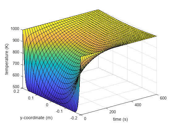
$Figure contains an axes object. The axes object with xlabel $y/b$, ylabel $\frac T-T indexOf 0 baseline T indexOf 1 baseline -T indexOf 0 baseline $ contains 9 objects of type parameterizedfunctionline, text. These objects represent $\tau=0.01$, $\tau=0.04$, $\tau=0.1$, $\tau=0.2$, $\tau=0.4$, $\tau=0.6$, $\tau=1$.$

Next, plot the temperature in the SI unit $K$ as a function of the $y$ -coordinate and time $t$ , where $T_{1} = 1000 K$ , $T_{0} = 500 K$ , $b = 0.2 m$ , and $α = 1 0^{- 4} m^{2} / s$ . Define these parameters and assume the units are in SI.

T1 = 1000;
T0 = 500;
b = 0.2;
alpha = 10^-4;

Define variables for the temperature $T$ , coordinate $y$ , and time $t$ . From the dimensionless temperature solution in Theta_sol, find the temperature solution in $K$ by substituting these parameter values. Also, replace the infinite summation terms with a summation term of up to $k = 40$ to improve the performance when plotting this solution.

syms T y t
T_eqn = (T1-T)/(T1-T0) == subs(Theta_sol,{eta,tau},{y/b,alpha*t/b^2});
T_sol = isolate(T_eqn,T);
T_sol = subs(rhs(T_sol),Inf,40);

Create a surface plot of the temperature as a function of the $y$ -coordinate and time. You can see that initially the slab is at $500 K$ with edges at $1000 K$ , and after about $600 s$ , the temperature across the slab reaches the steady-state value of $1000 K$ .

figure
fsurf(T_sol,[1 600 -b b])
xlabel("time (s)")
ylabel("y-coordinate (m)")
zlabel("temperature (K)")

Figure contains an axes object. The axes object with xlabel time (s), ylabel y-coordinate (m) contains an object of type functionsurface.

References

[1] Bird, R. Byron, Warren E. Stewart, and Edwin N. Lightfoot. Transport Phenomena, 2nd ed. (New York: Wiley, 2007), 376–378, Example 12.1-2.