Main Content

freqz

DWT filter bank frequency responses

Description

[psidft,f] = freqz(fb) returns the complex-valued frequency responses for the wavelet filters psidft and the frequency vector f for the discrete wavelet transform (DWT) filter bank fb. Frequencies are in cycles/sample or in Hz if a sampling frequency is defined in fb. The frequency responses are centered so that the zero frequency is in the middle.

example

[psidft,f,phidft] = freqz(fb) returns the complex-valued frequency responses for the scaling filters phidft for the DWT filter bank fb at all levels of the decomposition.

freqz(fb) plots the one-sided magnitude frequency responses for the wavelet filter bank, fb. Magnitude frequency responses are plotted for all wavelet bandpass filters and the coarsest resolution scaling filter. The legend is interactive. To toggle the visibility of the filter magnitude response, click the corresponding line in the legend.

Examples

collapse all

Create a DWT filter bank for a length 4096 signal and the Fejér-Korovkin fk22 wavelet. Plot the magnitude frequency responses of the wavelet filters and final resolution scaling filter.

len = 4096;
fb = dwtfilterbank('Wavelet','fk22','SignalLength',len);
freqz(fb)

Figure contains an axes object. The axes object with title DWT Filter Bank fk22, xlabel Normalized Frequency (cycles/sample), ylabel Magnitude contains 8 objects of type line. These objects represent D 1, D 2, D 3, D 4, D 5, D 6, D 7, A 7.

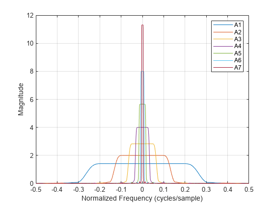
Obtain the frequency responses for the wavelet and scaling filters. Plot the magnitude frequency responses of the scaling filters at all levels of decomposition.

[psidft,f,phidft] = freqz(fb);
plot(f,abs(phidft)')
grid on
xlabel('Normalized Frequency (cycles/sample)')
ylabel('Magnitude')
legend('A1','A2','A3','A4','A5','A6','A7')

Figure contains an axes object. The axes object with xlabel Normalized Frequency (cycles/sample), ylabel Magnitude contains 7 objects of type line. These objects represent A1, A2, A3, A4, A5, A6, A7.

Plot the one-sided magnitude frequency responses of the wavelet and scaling filters at the first two levels of decomposition. Note how the second level frequency responses overlap the magnitude response of the first level scaling filter.

plot(f(len/2:end),abs(psidft(1,len/2:end))')
hold on
plot(f(len/2:end),abs(phidft(1,len/2:end))')
plot(f(len/2:end),abs(psidft(2,len/2:end))')
plot(f(len/2:end),abs(phidft(2,len/2:end))')
grid on
xlabel('Normalized Frequency (cycles/sample)')
ylabel('Magnitude')
legend({'Level 1 Wavelet','Level 1 Scaling', ...
    'Level 2 Wavelet','Level 2 Scaling'})

Figure contains an axes object. The axes object with xlabel Normalized Frequency (cycles/sample), ylabel Magnitude contains 4 objects of type line. These objects represent Level 1 Wavelet, Level 1 Scaling, Level 2 Wavelet, Level 2 Scaling.

Input Arguments

collapse all

Discrete wavelet transform (DWT) filter bank, specified as a dwtfilterbank object.

Output Arguments

collapse all

Wavelet filter frequency responses for the DWT filter bank fb, returned as an L-by-N matrix, where L is the filter bank Level and N is the filter bank SignalLength. The frequency responses are centered so that the zero frequency is centered in the middle.

Frequencies, in cycles/sample or Hz, returned as a real-valued vector of length N, where N is the filter bank SignalLength. If a sampling frequency is specified in fb, frequencies are in Hz.

Data Types: double

Scaling function frequency responses for the DWT filter bank fb, returned as an L-by-N matrix, where L is the filter bank Level and N is the filter bank SignalLength. The frequency responses are centered so that the zero frequency is centered in the middle.

Version History

Introduced in R2018a