mlptdenoise
Denoise signal using multiscale local 1-D polynomial transform
Syntax
Description
y = mlptdenoise(___,Name,Value)mlpt properties
using one or more Name,Value pair arguments,
and any of the previous syntaxes
[ also returns the thresholded
multiscale local 1–D polynomial transform coefficients.y,T,thresholdedCoefs]
= mlptdenoise(___)
[ also returns the original
multiscale local 1–D polynomial transform coefficients.y,T,thresholdedCoefs,originalCoefs]
= mlptdenoise(___)
Examples
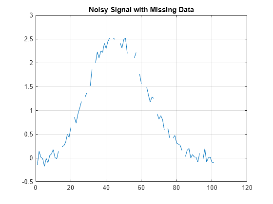
Denoise a nonuniformly sampled spline signal with added noise using median smoothing and two primal vanishing moments. The nonuniformity of the signal is indicated by NaNs (missing data).
Load the data to your workspace and visualize it.
load nonuniformspline
plot(splinenoise)
grid on
title('Noisy Signal with Missing Data')
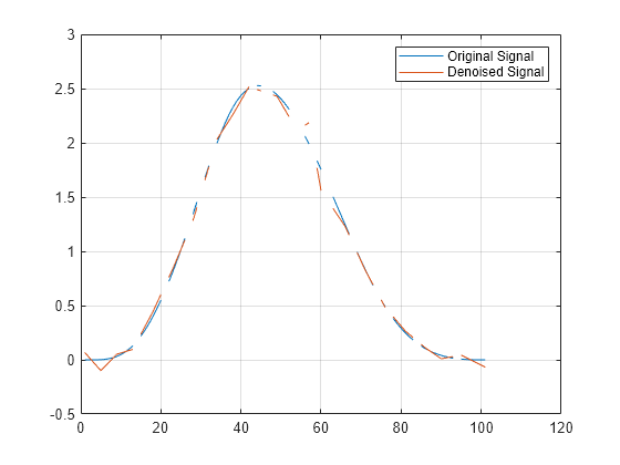
Denoise the data using the median denoising method.
xden = mlptdenoise(splinenoise,[],'DenoisingMethod','median');
Replace the original missing data in the correct position for plotting purposes. Visualize the original and denoised signals.
denoisedsig = NaN(size(splinenoise));
denoisedsig(~isnan(splinenoise)) = xden;
figure
plot([splinesig denoisedsig])
grid on
legend('Original Signal','Denoised Signal');
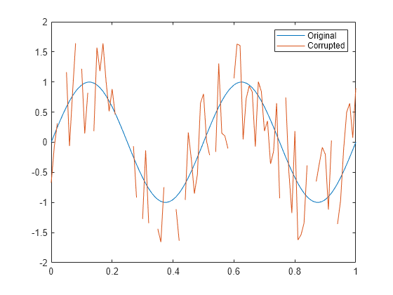
Reduce noise of signal using the multiscale local polynomial transform (MLPT).
Load a pure sine wave signal with uniform sampling, and a corrupted version of the signal.
load('InputSamples.mat')

plot(t,x)
hold on
plot(tCorrupt,xCorrupt)
legend('Original','Corrupted')
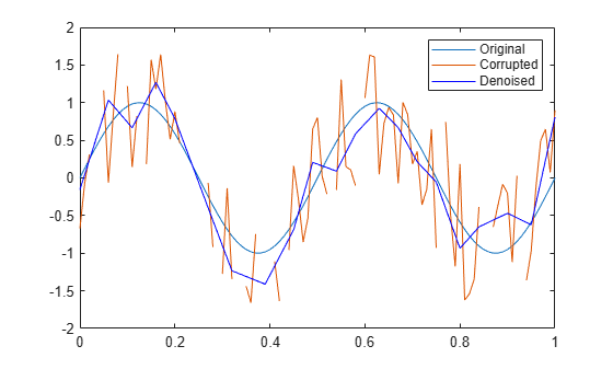
Use mlptdenoise to denoise the corrupted signal. Visually compare the corrupted and denoised signals against the original signal.
[xDenoised,tDenoised] = mlptdenoise(xCorrupt,tCorrupt);

plot(tDenoised,xDenoised,'b')
hold off
legend('Original','Corrupted','Denoised')
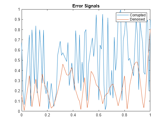
Compare the error signals associated with the corrupted signal and the denoised signal. Remove NaNs from the signals for visualization purposes.
x(samplesToErase) = [];
xCorrupt(samplesToErase) = [];

xCorruptError = abs(diff([x,xCorrupt],[],2));
yError = abs(diff([x,xDenoised],[],2));

plot(tDenoised,xCorruptError)
hold on
plot(tDenoised,yError)
title('Error Signals')
legend('Corrupted','Denoised')
hold off
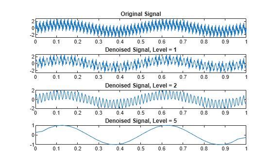
By default, mlptdenoise denoises a signal based on the two highest-level detail coefficients. In this example, you denoise a signal to different levels and visualize the effect.
Create a multitone signal.
fs = 1000;
t = 0:1/fs:1;
x = sin(4*pi*t) + sin(120*pi*t) + sin(480*pi*t);
Denoise the signal to levels one, two, and five.
y1 = mlptdenoise(x,t,1);
y2 = mlptdenoise(x,t,2);
y5 = mlptdenoise(x,t,5);
Visualize the effect of level on the denoised signal.
subplot(4,1,1)
plot(t,x)
title('Original Signal')

subplot(4,1,2)
plot(t,y1)
title('Denoised Signal, Level = 1')

subplot(4,1,3)
plot(t,y2)
title('Denoised Signal, Level = 2')

subplot(4,1,4)
plot(t,y5)
title('Denoised Signal, Level = 5')
The mlptdenoise function performs the forward MLPT, thresholds the coefficients as specified by the 'DenoisingMethod' name-value argument. Then mlptdenoise performs the inverse MLPT to return a denoised signal in the domain of your original signal.
You can optionally return the thresholded and original coefficients for inspection and analysis.
Denoise a nonuniformly sampled signal using Stein's unbiased risk method. Return the denoised signal, the associated time instants, the thresholded MLPT coefficients, and the original MLPT coefficients. Plot the original and denoised signals.
load nonuniformheavisine
[xDenoised,t,wThrolded,wOriginal] = mlptdenoise(x,t,3, ...
    'denoisingmethod','SURE');
plot(t,[f,xDenoised])
legend('Original signal','Denoised signal')

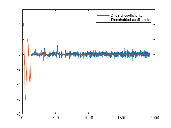
Plot the original MLPT coefficients and the thresholded MLPT coefficients for comparison.
plot([wOriginal,wThrolded])
legend('Original coefficients','Thresholded coefficients')
Input Arguments
Name-Value Arguments
Output Arguments
Algorithms
Maarten Jansen developed the theoretical foundation of the multiscale
local polynomial transform (MLPT) and algorithms for its efficient
computation [1][2][3]. The MLPT uses a lifting scheme, wherein a kernel
function smooths fine-scale coefficients with a given bandwidth to
obtain the coarser resolution coefficients. The mlpt function uses only local polynomial
interpolation, but the technique developed by Jansen is more general
and admits many other kernel types with adjustable bandwidths [2].
References
[1] Jansen, Maarten. “Multiscale Local Polynomial Smoothing in a Lifted Pyramid for Non-Equispaced Data.” IEEE Transactions on Signal Processing 61, no. 3 (February 2013): 545–55. https://doi.org/10.1109/TSP.2012.2225059.
[2] Jansen, Maarten, and Mohamed Amghar. “Multiscale Local Polynomial Decompositions Using Bandwidths as Scales.” Statistics and Computing 27, no. 5 (September 2017): 1383–99. https://doi.org/10.1007/s11222-016-9692-8.
[3] Jansen, Maarten, and Patrick Oonincx. Second Generation Wavelets and Applications. London ; New York: Springer, 2005.
Version History
Introduced in R2017a