Linearization of Upcoming High-Efficient RF Power Amplifiers, Part 1: Introduction to Linearization of RF Power Amplifiers for Wideband Applications

Welcome to our industry workshop. What's the title? Linearization of RF Power Amplifiers for Wideband Application. It's a collaboration between a good amount of different companies, Qorvo, MathWorks, MCAT, and Rohde & Schwarz. And at first, let me say, thank you to Georgia for setting this up, for making this all available, for herding us together, for bringing all of us together. So thank you very much, Georgia, for this one. Let's get started.

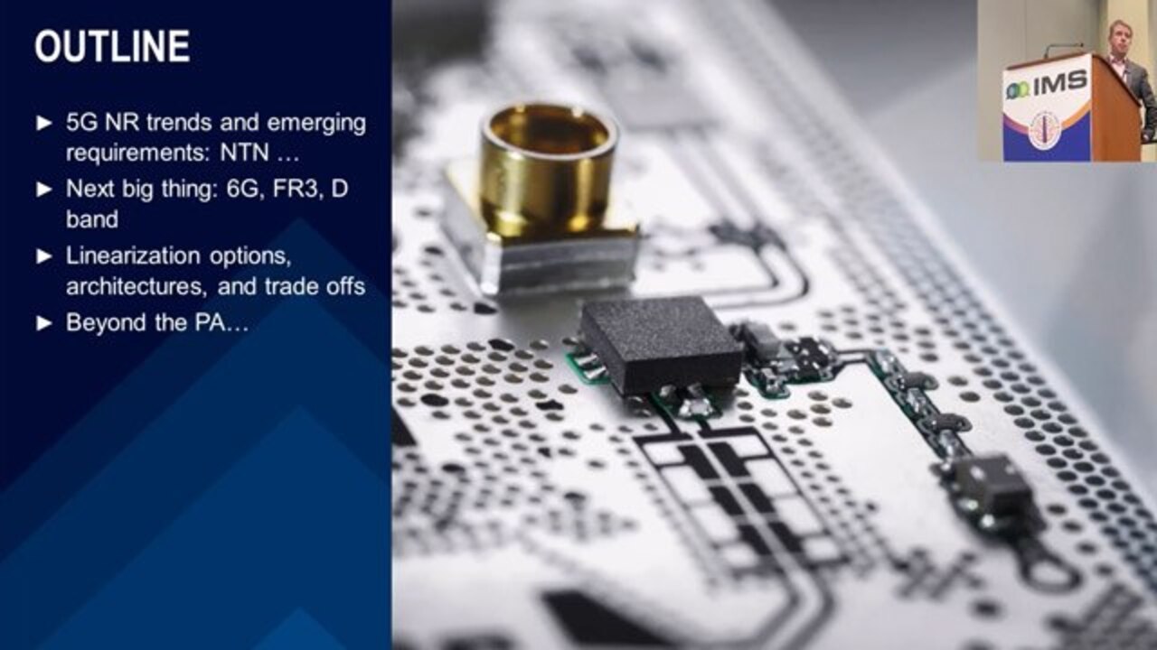
What do we want to talk about within the next 1 and 1/2 hours? At first, I will do a quick introduction of linearization of RF power amplifiers for wideband applications, as well as also give you some ideas about market drivers, what are current trends in the industry. Because in the end, all of those power amplifiers are made for certain target applications. And those target applications bring a good amount of different requirements with them. And that's why we want to have a quick start here at first.

Then we will have a look into dedicated technologies, efficient broadband power amplifier architectures for wideband applications, which will come from our-- from our friend from Qorvo. Thank you. And then, we're going to look into deriving PA measurement data from existing hardware for behavioral modeling and DPD, as well as PA behavioral modeling challenges for broadband applications. So basically, that's kind of a bringing together for MathWorks as well as for Rohde & Schwarz, and modeling and simulation of PA for digital predistortions applications.

So those are the three topics going a little bit closer in how to optimize with different techniques, and also where we compare simulation with real measurements, with real data, and where also MCAT comes into play in order to create an interesting model for using the data created before. All right, let's get started here.

What I want to talk about are some of the trends with regards to what drives our market. Obviously, there are different applications. The biggest one from a volume perspective nowadays is still the mobile communications in 5G. But there is also a lot of research and activity already going into the next generation, looking at 6G, looking at different frequency bands, but also, where is the differentiation in this direction? And the differentiation is not about, oh, I can support this frequency range. Or I can support this certain bandwidth.

No, the differentiation is in its efficiency. How efficient can I create a certain output power? And what is my power-added efficiency? And that's kind of also where we are looking at. And there are different techniques on one side, improving the design of the PA by itself using different topologies, but then also using digital predistortion in order to make a more efficient usage out of this.

All right. Beside the mobile communications, obviously nowadays, there is a lot of activity also going on in different topics. Mobile communications obviously going up at higher frequencies, talking to higher bands, research going up to D band activity, or even H band up in the 300 gigahertz range. But there is also a lot of research ongoing. And there's also a lot of sponsored-by-research activities with the CHIPS Act in North America, in Europe, and also in Asia.

Obviously, there is also quite some activities right now in the aerospace and defense, also with satellite communications. And those things are going to merge. I'm talking about that in a second. And last but not least, some automotive applications, because obviously, cars should getting more and more autonomous, which means they need to be connected. So they also need to have a certain connectivity there. I mentioned mobile communications satellite. They are coming together.

There is a term, which is called NTN, Non-Terrestrial Networks. In the end, it means your phone is talking directly to the satellite. It's an interesting subject. There is a common consensus that this is going to happen. This is going to be supported. But it's not defined yet how it should work exactly. The different network operators, the different Leo operators like a SpaceX or others. There is still a lot of debate, so to speak.

Nevertheless, what does this mean for us and the PA community? It will be a challenge in order to make a link really for that long distance, and also across different frequency bands. Talking about this, what is the possible deployment timeline? And there is already stuff happening today. Like, on the left-hand side, a narrowband application. And I have to say, I personally, I'm happy that this is already there because I live in Europe, I'm like to do some outdoor sports in the Alps.

If you're somewhere in a valley lost, there is no 5G, there is no 4G, there is no network connection. My phone shows me there is an SOS link to the satellite already today. So that's already in place. That's already working. So this is the emergency version on the left side. When we go in further to the right side, bottom line is increasing the amount of data rate and how can we connect there, as well as how much can we go into a more compact version, into a more compact device?

And yes, you kind of see when you look at the time schedule, that pretty much goes towards almost want to say the end or just towards the start of the next generation 6G, which is kind of foreseen for the 2030s range. I mentioned before, there is a lot of stuff still open. The specifications look at different frequency bands. And it's going all across the map from FR1 bands to FR2 bands, FR3, and even higher. So that will be quite an interesting topic, depending on the different use cases, depending on the different bandwidths which should go through.

And on the right side here, it just gives you also some of an indication what type of power levels are to be expected, are to be reached. Also with regards to for some receivers, what type of noise figures? And those are pretty demanding numbers already. The other topic was NTN as it's really sitting inside of the traditional mobile comm bands. You have to be careful about sideband thickness, which come out. So the traditional ACLR measurements, as we know it from the mobile applications, will also be important in NTN because those will sit right next to each other band wise.

That being said, you have to be careful for coexistence. And I mentioned before 6G as a topic, well, I think everyone has seen before that 5G triangle in the end in 6G, they want to extend it from three different corners to six different corners was integrated at AI ubiquitous connectivity, as well as integrated sensing and communication, which drives also usage, or it gives application for higher frequencies, especially those sensing-- integrated sensing and communication.

HG recognition is another topic, which is kind of being talked about this. Obviously, there will be also the counterpart for coverage and all of those things. So when you look at the different topics for 6G, yes, a lot of discussions is right now going on into higher frequency ranges like D band tera, sub terahertz topics. There is also FR3, another new frequency band in between FR1 and FR2.

But to be really clear, there will be a lot of still applications also in the common FR1 band. So the PA designs, as we do it today, will be able to be reused also in the 6G to a certain degree needs to be adopted. But the frequency range in the FR1 will be still available because that's the only way to really do coverage.

FR3, just a quick glimpse on that one. It's basically the band in between FR1 and FR2 in the standardization. Sometimes called FR3, sometimes called FR2-0 because it's the lower extension to it. Why is of interest? Because you could pretty much reuse technology from FR1, drive it up higher frequency, and for example, in the filter world, you already see more acoustic filters being used in that frequency range. It's being driven up to that range.

And from a PA perspective, it's kind of in the same idea to use similar concepts. There are discussions in FR3 if it should be a full beamforming system versus a broadcast system. I think there will be a combination of both. As we are talking about really high frequency also in the D band, just a quick look of new stuff, which we are also including within Rohde & Schwarz to reach those sectors. I don't want to go into detail. If you want to see stuff, like this live, just come by our booth, and we are happy to show you.

Talking about optimization using different PA topologies. There are different things. Number one, with a PA, you have to-- with a front end, you have to sign up for certain numbers for certain performance, things like the frequency range, the output power, the signal performance. That's defined and given by the standard. The differentiator is the efficiency. And there are different methods to do that.

One is to look at the different classes, different types, topologies of amplifiers. And I kind of like that approach because it kind of looks a little-- it kind of shows a little bit like the different techniques to enhance those power amplifiers. And we classified it in traditional waveform engineering like class A, class B, et cetera.

Then supply modulation, which is a typical thing used in mobile devices with envelope tracking, for example. And last but not least, load modulation, which comes into other topics where we see Doherty kind of being a part of it or LMBA topologies, where also, actually will talk a little bit more in closer detail about it.

Linearization. Why is this a necessity? Bottom line, signals are getting pretty demanding. Higher frequencies, higher bandwidth, massive MIMO, beamforming. They all want to do high-bandwidth signals as linear as possible, but still very energy efficient, because actually, the majority of power in a mobile phone, in an infrastructure, is consumed still in the front end in the amplifier. And certain technologies like GaN, they almost require, by default, any kind of a predistortion, and different topologies allow also different methods to combine.

So there is not like, you just do one side, and everything will be good. No, you basically want to combine the different approaches with topologies on one side, and using predistortion on the other side in order to make the amplifier more efficient, more linear at higher output power levels. So in the end, linearization is very often a must in order to extend the linear range by making the traditional nonlinear behavior linear. Why? Because when we look at this plot on the top right, ideally, we want the red curve, which is a very linear plot.

Reality is at a certain point, our front end goes into saturation, and it's not that linear anymore. And so the input signal versus the output signal gets some distortion up here. Predistortion is nothing else than to kind of preequalize-- the input signal to precompensate for what is happening here with an input signal, as you see up there. Goal is to keep it as long as possible linear until it kind of hits a brick wall, and you are at the maximum output power what can be achieved.

Typically, it's something like a closed loop as you see it down here. And below, you see a possibility how to verify how to test this. Why are we using digital predistortion? Why do we have to do this? Because our front ends are the most efficient the closer we get to saturation. The closer we are at saturation, the better the power added efficiency becomes. But they are non-linear. So you want to push them into it, but you have to pre compensate for this non-linear behavior.

All right. Giving a quick optimization options summary here. It is very much dependent on the target application. So if you're doing just a rate of CW pulse, you can drive the amplifier basically into compression. Nobody cares. All good. But if you're doing modulation, that's not the right approach because then, there is no crest factor. It's all gone. So you need to go back a little bit. How far? That's another game. And to keep it still linear up there, that's where digital predistortion comes into the game.

Talked about the efficiency. That's obviously made for lowering power consumption, but also for thermal management. So the more efficient the whole front end gets, the easier it also becomes with power with cooling, which can be also a thermal effect on the front end, which needs to be covered on one side, but also on the other side consumes power.

OK, I think I talked about dosing on the right side. Bottom line, there is not a, I just do one approach and I can use it for any different applications. No. I have to look at my use case and then adopt the topology as well as the linearization approach according to this.

The other thing, when we are defining amplifiers, probably to step a little bit further outside of the box, when we're defining amplifiers, we need to drive typically any signal over the air for any communication. Could it be any radar signal, could be any communication signal, any satellite link. When we are talking about antennas at a linear, at a flat, at 50 ohms, not really. Whenever we test something, or whenever we work with most of the stuff, we are assuming a 50-ohm world.

Unfortunately, the world is not 50 ohms. Yes. In modeling, we are doing a lot of stuff with looking into the behavior across different impedances. But while making measurements, we are typically looking at 50 ohms worlds. And I think that this is also the maturity in simulation. But reality means, especially when you have a one antenna which covers a wider bandwidth, it's not a 50-ohm world. It's probably something going from 10, 15 ohms, all the way to 150 ohms, with just a wide bandwidth coverage.

And the problem is that our front end behaves differently if you have 50 ohms, 80 ohms, or 30 ohms. How to verify this. You cannot predict it. That's the problem. So you need to look into measurements at different impedances. And yes, traditional load pool is doing that very nicely for a CW signal. Is this always a valid approach? Not really. In many applications, the wider the bandwidth you-- and the more complex the modulation, You should also do this. You need to do this basically to understand ACLR is still met. So no sideband signal.

You need to measure this also within a modulated approach. And we have just-- we are just in the process of developing, of designing a new project, which is doing exactly this measurement with different impedances. Bottom line, it's an active load pull system supporting modulated signal, no matter which bandwidth. Could be 5G, could be satellite links, could be 6G, whatever.

Just a quick teaser. We have it also in our booth. It's now as a beta stadium, a proof of concept right now. And we are also looking into how can we extend this to higher frequencies into the millimeter wave range, et cetera. But it's a very interesting topic to really ensure that your PA not only works in the simulated and 50-ohm world, but in the real environment. You are seeing wide ranges of applications. And that's exactly what this is doing.

And when we talk about validation of PAs and everybody is talking about ACLR and easy, even there are different methods. People are looking at EVM and understand different topics. Very easily to be separated, there is a standard compliant on the right side. So if you're measuring something really according to a standard, it's doing a true demodulation. There is the other topic, the other measurement, which is called an RMS EVM. What difference is that on one side, you really demodulate the signal. You look for the signal where is the closest constellation diagram, and calculate the difference.

RMS is going a different approach. It really compares the INQ sample of the transmitted versus the received. And that's the difference of that one. So there are two different approaches, which can also lead to certain variants in the results. Interestingly, in the end, the RMS EVM is giving you the more accurate number because it really compares input versus output. OK. With this one, I want to hand over to Salva.