Development of CRM for Reservoir Simulations Using PINNs | MathWorks Energy Conference 2022
From the series: MathWorks Energy Conference 2022
Mark Behl , Chevron
Mayank Tyagi , Lousiana State University
Reservoir simulators play a key role in the management and optimal production from oil and gas fields. However, the computational costs of detailed simulations can be prohibitively expensive and most certainly not useful for real-time decision-making. In this presentation, a reduced-order model (ROM) is built using the time-series production data from a real oil and gas field. The CRM is chosen here as a reduced-order representation for the reservoir simulator.
With the increase in computational power and recent machine learning (ML) approaches, it is apparent that the oil and gas industry will eventually adopt useful models through proper validation. PINNs are the neural networks that can enforce the governing equations for the underlying dynamics as a part of building ML models. Results are compared against a detailed reservoir simulation to demonstrate the usefulness of ML models.
Published: 22 Mar 2023
Hello, everyone. It's my pleasure to present our research work on the development of capacitance resistance models for reservoir simulations using PINNs, also known as Physics Informed Neural Networks.
It's a pleasure to introduce my team members. Mark Behl, who works at Chevron, and this is his master's thesis work. And Dr. Oscar Molina, he works at MathWorks. And he's going to be taking it forward further in the future collaborations. So the floor is yours, Mark.
Hi, everybody. My name is Mark Behl. I'm a production engineer with Chevron. And the topic of this discussion, like Dr. Tyagi said, is development of CRMs for reservoir simulation using PINNs. So it's a lot of flashy words to unpack. But the main idea behind the talk is to explore development of lightweight reduced order models for oil and gas reservoirs as an alternative to traditional numerical simulation.
So through this talk, I'll share with you some of the novel machine learning techniques I explored during my graduate research, and show you the potential to accurately forecast production, validate results against real historical field data, and then further improve the results by applying a physics based constraint to the model.
So to start, we'll begin with a description of the problem statement and the data. I want to take a minute to acknowledge Equinor for providing all the data used in this study, the production data in the reservoir simulation model are part of the Volve data set, which Equinor released around 2018 after the field was decommissioned.
It's unusual for the oil and gas industry to share that volume of data. So we really appreciate it and hope to see more of it in the future. After we talk about that, I'll try to give not too hand wavy the overview on LSTM neural networks and capacitance resistance models.
After that, we'll show how I coupled those techniques and apply them to the Volve data. And after sharing results, I'll turn it over to Oscar, who will talk about work that he's currently doing moving forward on this.
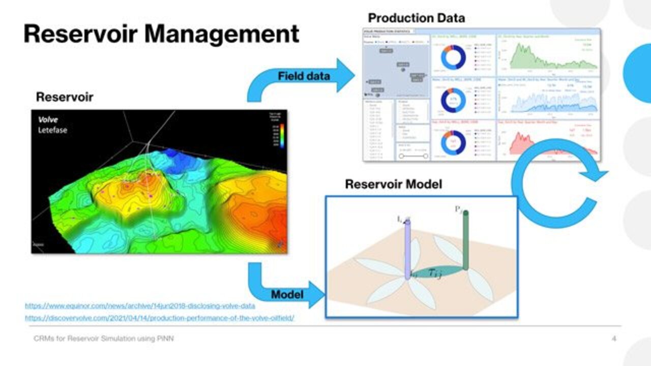
So this is the Volve field on the left. It's in the North Sea. Like I said, was produced by Equinor from about 2008 to 2016. You could see it's not a very big field. There's two water injection wells and five producers. And in the upper right, you see the time series of the rate histories for the oil, water, and gas.
So when we talk about reservoir management, we're trying to optimize the hydrocarbon recovery by monitoring those wells' performance, and then adjusting our field strategy according to how we approximate the current reservoir conditions.
So traditionally, the gold standard for that reservoir characterization is using a grid based simulation model, in which we try to reconstruct the subsurface environment based upon a geologic interpretation of seismic data or rocket fluid properties. And then we calibrate the model by solving governing equations for this simulator, some form of conservation of mass, and then we history matched to those scene rates.
So like I said, this is the all-inclusive proven technology for the full field characterization. But it's really computationally expensive. It's time consuming and super inefficient for real-time decision making.
So because we have the measured data at the surface, what if we could simply redefine the reservoir as control volumes between injector and producer payers? Cut out a lot of that uncertainty, and I don't want to say unnecessary data, but come to roughly the same conclusions on the production performance of the wells with that reduced order model.
So if you wouldn't mind pulling up those slides, Dr. Tyagi. On the left, we see the governing equations for the traditional black well simulation model. You can see for each of the three phases seen in the reservoir, the oil, the water, and the gas both in solution, and in the free phase we essentially have to solve the conservation of mass and momentum for each of those phases for every single grid block, and for a field the size of Volve that can be around a million calculations per time step.
And then in addition, we also have the well component, where you see Q, formula, and the productivity index, which is just the ratio of that fluid rate to the pressure drawdown required to hold that rate constant.
So again, tons of calculations needed, very computationally expensive. So as an alternative to the right, you see what I started talking about, what we call the capacitance resistance model. And this model actually predates grid based simulation.
There's a really cool study back in the 1950s, where they proved there's an analogous relationship between fluid flow in porous media and the flow of electricity in a circuit. So in the same way that a circuit can store that electricity in a capacitor, the reservoir has the ability to store that energy due to the compressibility of fluid.
And then, the same way there's a resistance in that electrical network in the reservoir, there's that resistance to flow. It's related to the inverse of the transmissibility of the reservoir. So by moving to this reduced order model using the CRM, instead of having however many equations for however many millions of grid blocks, we're able to reduce it down to just a few unknowns for each injector producer pair.
So the tau that's shown, that's the dissipation coefficient. And that's just the dissipation of response between the pairs. F is the fractional volume between those control volumes. And then again, J is the productivity index for that specific control volume. So we're assuming that for each injector producer payer, the corresponding injector is the only injector acting on that volume and the rate that producer produces corresponds solely to that injector.
So when we start with just the statistics and show plotting the Pearson correlation coefficient, you can immediately see that there's a strong correlation. I'm looking at injector 5, and you can see a good amount of that injection rate can be contributed into Producer 12 and 14.
So next, I'll talk about the structure of the networks that we use. Because we're using only the surface rate data that we measured, we lose a lot of the reservoir. But the temporal structure of that data is also a feature that we can exploit.
So in this work, we use long short term memory networks, which are a form of a recurrent neural network. Those differ from what they call vanilla neural networks, just a multi-layer perceptron, in that recurrent networks are able to retain a memory of the previous input.
And we use LSTM as opposed to just a traditional recurrent neural network, because we're trying to exploit that long rate history of the well and see if we can learn more from the historical data, because some of the producers go back eight years. So there might be more information we can glean, instead of losing information from just the previous time step, or having to deal with vanishing gradients as we're training the network.
Now, in work, we recognized, again, that there's GRUs and there's other alternatives. But this was a specific one we chose for this work.
Now, using the LSTM to predict, there's other literature that already shows its validity for use in production forecasting. But there's a technique that's not used very widely in the petroleum industry, but is pretty new and pretty cool, I think.
Neural networks have a reputation as sort of a black box. They're really good at solving the problem of where we try to learn the mapping function from the input to the output. But then we don't really have a whole lot of inference into how it's doing that or what else it's telling us.
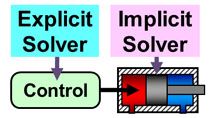
So there was-- it's with the Brown crunch group, Rice and Carnegie came up with what they call a physics informed neural network. And what that does is you apply a respective differential equation that kind of defines the defines the system. It's used as a regularization technique to constrain a solution space to meaningful results.
So instead of just having a number solver, we're putting a little bit more control on there to something that's physically plausible. So the way that works, with that CRM equation that we saw, you feed in the rate data and then we use the downhole pressure data from just the producers, not the injectors.
And you feed it into the LSTM network, and that predicts the specific rate contributions for each injector producer pair. So we're only feeding it five production inputs, two injection inputs, and then the five bottom hole pressures. And its outputting 2 by 5, so 10 injector producer pair rates. And then it feeds it into almost a second network, which uses automatic differentiation to find the rest of the equation, to find the derivative with respect to time.
And then we use external sensors for the tau, the F, and the J for each component. And then use that to apply to the loss. So instead of just having the loss be the difference between the prediction and the output for the rates, we have the added loss from solving the differential equation. So it penalizes it a little bit more. But it has the added benefit of it's also solving the ideal parameters that describe the system.
So here we see just the typical 60/40 split. I used Producer 12 to train on monthly data, and then predict for the last bit of it. And you can see it performs really well. And then to the right, we compare it against the output from the simulator. And you can see that the LSTM network with monthly production data alone for a single well outperforms the reservoir simulation.
And then once that was trained just on PF 12, we were able to apply that same trained network and feed it production data for the remaining four wells. And you could see, again, the volumetric error between the two. It continued to outperform the reservoir simulator.
So the results we just saw were for the single well models. That kind of fell apart when we tried to throw it as all inclusive model for the field. You can see an image on the left where it's highlighted in red. The network predicted negative rates.
So it's not plausible results. The prediction error was fairly low. But it doesn't make any sense. So to the right, you can see, by adding the constraint of the CRM equation, it constrained the problem into meaningful results. It cut down on the error and we were still able to attain the same kind of accuracy.
So this plot shows the results for those governing equations that it solved for each injector producer payer. The image on the left is for, again, the taus, the dissipation coefficients. And this one I was especially happy to see, because it's kind of unusual results.
So the vectors that are shown or the thicknesses showing the magnitude of the dissipation coefficient. So normally, as you can see coming from Injector 5, the further away the well is, you would expect a larger coefficient. And if you look at Injector 4, the one on the bottom, the vector pointed towards producer F1C. In the far upper left is a surprisingly small dissipation coefficient.
And that is unexpected with the distance and having the other wells in between. And you can see on the right, when we use the full blown simulator to plot the streamlines, that there's good agreement between the two.
So all in all, I think just on a proof of concept level, the network is not fully optimized by any means. This is probably not a unique ideal solution, but just qualitative results showed really good agreement early on.
All right, Mark. So yeah, I think your results look very interesting, for everybody watching this presentation, CRM model has proved to be really robust model. And as Mark mentioned, even though there are some improvements to be made on the model, there are still some current challenges that need to get addressed. And that's where I kind of like join Professor Tyagi and Mark's research in the area.
So one of the nicest things that we saw about the CRM approach or the team approach is that it's a very nimble model, very lightweight, but it's very efficient, right? So we want to retain that efficiency in order to forecast production.
And that's a challenge, because the model is using data-- it's utilizing production data in order to regress the set of equations using the LSTM network. And then based on that, we kind of see how the model performs with known data. But it's limited in time.
Now, what we want to do is how do we forecast, how do we use that model to forecast production into the future? And like CRM models perform really well with mature aggressive work. That's what we call a Brownfield, where we have a very well established number of wells, both injector and some producers.
But in the process like showing wells in like, for example, the productivity level of some wells have dropped below the economical levels. So operators will just go and shut them in. So for the model, it's like a well had just disappeared. And the model might not be trained to handle those situations. And the same is true when you add new wells into the field.
So for example, if the operator wants to increase production by just drilling uncompleted new infield wells. So the model doesn't know about these new wells, and then this is where we might encounter some problems.
And of course, there are aspects of using CRM for full analysis. One of them is that, at the moment, as Mark mentioned, the model is focused on what's happening in the subsurface, right? So we use data at the surface to try to understand what's going on in the subsurface.
But nothing said about how the wells interact with one another at the surface level. So that's one of the challenges that we seek to address in the near future.
And the other one is to include economics into the analysis. So far, we have talked about history matching pressures-- rates, excuse me, then forecasting. But then how do we tie it up with economics at the field scale.
So what we're currently doing with MATLAB is that we are taking advantages of-- we're taking advantage of the way that Matlab plays with commercial cloud computing solutions like Azure and AWS, because all of those APIs are readily available in MATLAB code. So we just call a function and we connect, we get connected with Azure, with AWS.
MATLAB also plays really nicely with other open source solutions like Python. We can also import SQL databases and analyze that data inside of MATLAB. So we don't have to go elsewhere, so the data stays .
The other advantage is that MATLAB has a LSTM model, a built in LSTM functionality that we can take advantage of. So all of the automatic differentiation, all of the network building functionality is already there. So we can just grab it from code MATLAB and just use it, right?
We also have the optimization toolbox, so we can make improvements with optimization process through the regression process. Especially if we want to do this by hand, as Mark mentioned, we have to put some constraints that the model will not naturally see. And that's where the optimization toolbox can be very handy.
And finally, we have MRC, which is a numerical simulator that was built into-- it's a native MATLAB simulator, so we can use it as our numerical simulations .
And of course, MATLAB will be at the center of it all. And then this will become sort of a closed loop solution for the rest of the management aspect of the model piece of it. So with MRC, what we're looking at is to be able to simulate complex models like the one that I'm showing you right here, where you have, you know, developed properties vary across the field or across the reservoir. So it's not an easy case to handle anymore.
The advantage of having MRC available there in MATLAB is that we can just put a number of wells right there, shut them in, drill new wells, simulate massive shut ins, and see how the LSTM model will react to those changes. So we will be able to train the model, the team model more effectively, because MRC is available right there in MATLAB, so that we can have that as an integral part of the workflow.
And the other part that Mark mentioned in the beginning is data management, right? So a producing field can-- will definitely produce a vast amount of data. So big data would likely become an issue. And MATLAB plays really nicely when it comes to big data. And actually, we have a full presentation on that, that I will leave you a link of your presentation to that discussion on our website.
So taking that into the real time domain is the next phase. So what we want to do is to take and convert the CRM model, the PINN model, into a reduced order model. And again, as I mentioned just a minute ago, the challenge here is to forecast production, right? We can feed the model with almost real time production data using, for example, an OSISoft PI system, right? So we feed that down into the model, we run the prediction.
But then how can we forecast production based on that or near real time model? And then tie it up to an economic target. So for that we plan to use the Optimization Toolbox in order to close the loop. And then if you notice, we have that arrow tying up optimization algorithm with production operations. So this is when IoT devices come into play.
And finally, the next challenge is what are dynamics. So I mentioned that connecting the wells or converting data from one point to the surface, which is where we usually get pressure data. It's very rarely that the situation where we actually can get real time quote unquote pressure data, right?
So we most commonly will get pressure at the surface. So how do we convert that pressure to downflow conditions? And that's the next challenge that we are addressing. So there are two ways. One is using a physics based model, which uses-- where we solve the traditional conservation laws-- mass, energy, and momentum.
And we can also do a data-driven approach in which we can apply a similar approach that Mark presented today, but this time for . So that way, we create a model that is nimble enough to be coupled up with the PINN model, and then get a very fast and get accurate representation of the field, including surface conversion.
With that, I'm going to leave, Dr. Tyagi, and give his closing remarks about this presentation.
Well, thank you, Mark. Thank you, Oscar. So in this presentation, we have been able to demonstrate that LSTMs are useful machine learning models, especially for the time series production data, from that is demonstrated on the field case of well. And they also helped in developing some reduced order models that, of course, as decision-making tools for the reservoir management.
In particular, we showed that the PINNs constraint provides both physics informed and interpretable machine learning models for the subsurface transport between the well pairs. And like Oscar mentioned, it is in the future work that we are also using MATLAB as an integration platform to connect between the reservoir management workflows with all the cloud services and the IoT devices.
In the future, we will also extend the LSTM model for different productions forecasting scenarios and other type of machine learning techniques. And in our second talk, we were talking about data-driven ins models. For this work, we would like to acknowledge the generous licenses that are granted by CMG, for which we made sure the streamlines patterns match support for Mark, from the Craft and Hawkins Department of Petroleum Engineering, and all the data that was provided generously by Volve and Equinor.
And these are the most useful references regarding the LSTMs, the CRM, PINNs, all field data, as well as MRST, which is the reservoir simulation tool in MATLAB. With that, we thank you for your attention, and we'll take your questions when we will be presenting this research in person. Thank you, all.
OK. So time.
Do I post this, Dr. Tyagi?
Oh, I'm just stopping. 25 minutes. It's a little slow. But what I would say is I'm just going to quickly look at it. I think it turned out OK. It's good to have between 20, 25 minutes and 5 minutes. They are giving us 30 minutes, right?
Yeah, that's right.
Yeah. So what we will do is when we are going to do it in person on Thursday, it's OK that we shave off a little bit of our discussion. I enjoyed listening to you-- because you can't assume the audience. So Mark, I think you did fantastic. Both of you. You hit all the points correctly.
Related Products
Learn More

Featured Product
Simscape


Select a Web Site
Choose a web site to get translated content where available and see local events and offers. Based on your location, we recommend that you select: United States.
You can also select a web site from the following list
Americas
- América Latina (Español)
- Canada (English)
- United States (English)
Europe
- Belgium (English)
- Denmark (English)
- Deutschland (Deutsch)
- España (Español)
- Finland (English)
- France (Français)
- Ireland (English)
- Italia (Italiano)
- Luxembourg (English)
- Netherlands (English)
- Norway (English)
- Österreich (Deutsch)
- Portugal (English)
- Sweden (English)
- Switzerland
- United Kingdom (English)