Reconstruction of 3-D Radiation Pattern from 2-D Orthogonal Slices
This example shows how to reconstruct a 3-D radiation pattern using patternFromSlices function. A 3-D radiation pattern is a very important tool for antenna analysis, characterization, design, planning, and applications. This example shows reconstruction of 3-D radiation pattern from two orthogonal slices for an omni-directional dipole, a directional helix, and imported pattern data of an antenna.
Create Omni-Directional Dipole Antenna
Define an omni-directional antenna such as a dipole with a specific frequency and required elevation and azimuth angle.
ant = dipole;
freq = 70e6;
ele = -90:5:90;
azi = -180:1:180;
Generate Orthogonal 2-D Slices for Dipole
The slice is along the vertical direction using patternElevation function. Here we can give other 2-D pattern data as well.
vertSlice = patternElevation(ant,freq,0,Elevation=ele);
theta = 90 - ele;
Visualize the two orthogonal slices.
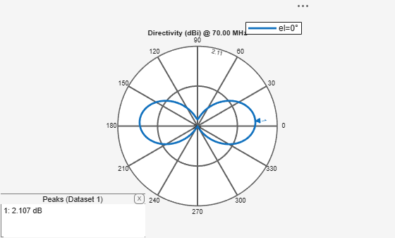
figure
patternElevation(ant,freq,0,Elevation=ele);
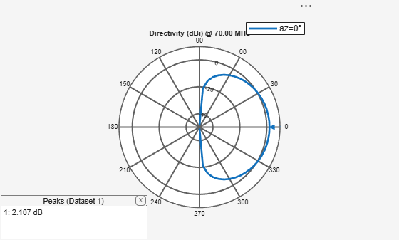
figure
patternAzimuth(ant,freq,0,Azimuth=azi);
Reconstruct 3-D Radiation Pattern of Dipole
For an omni-directional antenna, you can reconstruct the 3-D pattern using vertSlice alone. When only the elevation pattern data is provided, function assumes omnidirectionality of the antenna with symmetry about the z-axis (i.e. azimuthal symmetry).
patternFromSlices(vertSlice,theta);
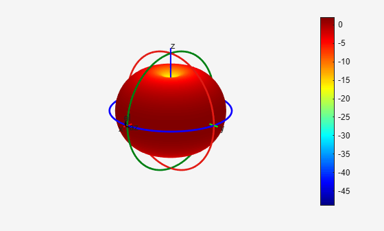
Reconstruction using both vertSlice & horizSlice data points can also be done for the above case. The reconstructed pattern does not vary. Thus for any omni-directional antenna, a 3-D pattern can be reconstructed with enough data points from orthogonal slices along the theta direction. The reconstructed radiation pattern looks like the 3-D radiation pattern which can be obtained using the pattern function.
Automatic Discarding of Data Points
Discarding of data points during reconstruction of 3-D pattern happens when both data points span across 360 degrees in 2-D plane. Since the algorithm needs a maximum span of 360 degree in one plane and a span of 180 degree in the other plane, extra data points are discarded.
vertSlice = patternElevation(ant,freq);
theta = 90 - (-180:1:180);
Dimension of pat3D is not equal to the length(phi)*length(theta) in this case. The size of thetaout also varies from that of theta dimension. Also, thetaout data shows the values for which data points have been considered during reconstruction.
[pat3D,thetaout]=patternFromSlices(vertSlice,theta);
Warning: Vertical pattern slice data from backplane for theta greater than 180 degrees is discarded.
dim_theta = size(thetaout);
disp(dim_theta);
1 181
3-D radiation pattern is not affected by the discarded data since there are enough data points along both the orthogonal planes for reconstruction of a 3-D pattern. This result is similar to the above reconstructed 3-D radiation pattern.
patternFromSlices(vertSlice,theta);
Warning: Vertical pattern slice data from backplane for theta greater than 180 degrees is discarded.

Directional Helix Antenna
Define a directional helix antenna with an operating frequency of 2 GHz. Define azimuth and elevation angles.
ant_dir = helix(Tilt=90,TiltAxis=[0 1 0]);
freq = 2e9;
ele = -90:5:90;
azi = -180:5:180;
Generate Orthogonal 2-D Slices for Helix
Calculate the directivity values along the vertical slice using the patternElevation function.
vertSlice = patternElevation(ant_dir,freq,0,Elevation=ele);
theta = 90 - ele;
Calculate the directivity values along the horizontal slice using the patternAzimuth function.
horizSlice = patternAzimuth(ant_dir,freq,0,Azimuth=azi);
phi = azi;
Visualize the two orthogonal slices of the directivity plot.
figure
patternElevation(ant_dir,freq,0,Elevation=ele);
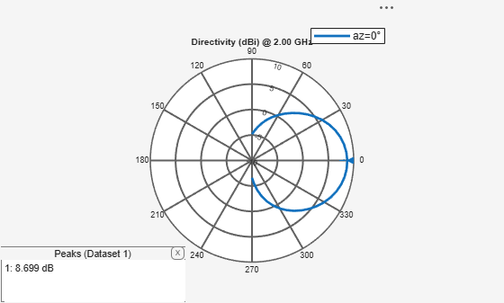
figure
patternAzimuth(ant_dir,freq,0,Azimuth=azi);
Reconstruct 3-D Radiation Pattern of Helix
For a directional antenna pattern, both the horizontal and vertical slice must be provided for accurate pattern reconstruction. Two separate algorithms are implemented for pattern reconstruction as below.
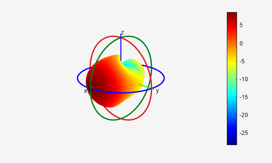
Summing Method
The "classic" summing algorithm is the default method. This algorithm can be used for near-perfect reconstruction of omni-directional antennas than for directional antenna.
patternFromSlices(vertSlice,theta,horizSlice,phi);
CrossWeighted Method
In this algorithm, the normalization parameter can be changed to obtain different results for the reconstructed pattern about the estimated directivity/gain.
patternFromSlices(vertSlice,theta,horizSlice,phi,Method="CrossWeighted");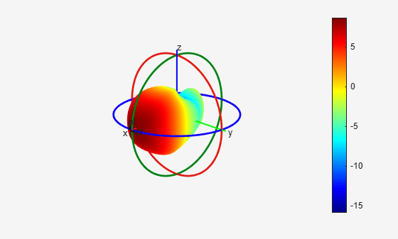
Visualize 3-D Radiation Pattern Using pattern Function
Visualize the original 3-D radiation pattern of the helix antenna using pattern function.
figure
pattern(ant_dir,freq);
By comparing the 3-D radiation pattern using pattern function with the reconstructed 3-D radiation pattern, it is clear that the front plane of the 3-D pattern is reconstructed well compared to its back plane. Also, reconstruction done using the CrossWeighted method is more accurate than the summing method in this case.
Read and Visualize Antenna Data from Manufacturer
Antenna manufacturers typically provide details of the antennas that they supply together with the two orthogonal slices of the radiation pattern. The pattern data is available in a variety of formats. One such format supported in the Antenna Toolbox™ is the MSI file format (extension .msi or .pln). Use the msiread function to import the data into the workspace.
[Horizontal,Vertical,Optional] = msiread("Test_file_demo.pln");Adjust dBd Values to dBi
If the imported data is in dBd unit, convert it to the dBi unit.
if strcmpi(Optional.gain.unit,"dBd")
    Horizontal.Magnitude = Horizontal.Magnitude + 2;
    Vertical.Magnitude = Vertical.Magnitude + 2;
end
Visualize Manufacturer data Using Polar plot
Visualize the vertical and horizontal gain data in an interactive 2-D polar plot.
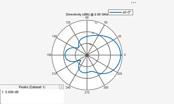
figure
P = polarpattern(Vertical.Elevation, Vertical.Magnitude);
P.TitleTop = "MSI Planet file data";
createLabels(P,"az=0#deg");
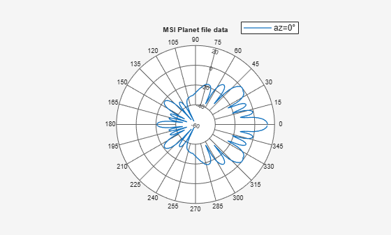
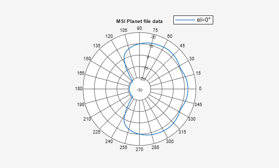
figure
Pel = polarpattern(Horizontal.Azimuth, Horizontal.Magnitude);
Pel.TitleTop = "MSI Planet file data";
createLabels(Pel,"el=0#deg");
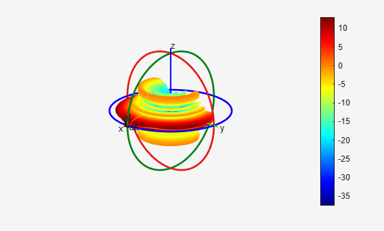
Reconstruct 3-D Radiation Pattern from Manufacturer Data
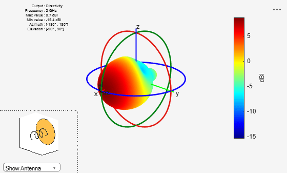
Extract the pattern slice magnitude data from the two output structures as well as the azimuth and elevation angle data. Note, that the angle data must be adjusted for the phi-theta convention. The azimuth angle maps to phi but the elevation angle is adjusted by 90 degrees to map to theta. See the Antenna Toolbox Coordinate System for more information.
vertSlice = Vertical.Magnitude;
theta = 90-Vertical.Elevation;
horizSlice = Horizontal.Magnitude;
phi = Horizontal.Azimuth;
patternFromSlices(vertSlice,theta,horizSlice,phi,Method="CrossWeighted");
Warning: Vertical pattern slice data from backplane for theta greater than 180 degrees is discarded.
See Also
Objects
dipole|helix|polarpattern