helix

Create helix or conical helix antenna on ground plane

Description

The default helix object creates a helix antenna on a circular ground plane resonating around 1.56 GHz. You can also create a conical helix antenna by specifying vector values in the Radius property. The helix antenna is a common choice in satellite communication.

The width of the strip is related to the diameter of an equivalent cylinder by the equation

$$w=2d=4r$$

where:

• w is the width of the strip.

• d is the diameter of an equivalent cylinder.

• r is the radius of an equivalent cylinder.

For a given cylinder radius, use the cylinder2strip utility function to calculate the equivalent width. The default helix antenna is end-fed. The circular ground plane is on the xy- plane. Commonly, helix antennas are used in axial mode. In this mode, the helix circumference is comparable to the operating wavelength and the helix has maximum directivity along its axis. In normal mode, the helix radius is small compared to the operating wavelength. In this mode, the helix radiates broadside, that is, in the plane perpendicular to its axis. The basic equation for the helix is

$$\begin{array}{l}x=r\cos (\theta )\\ y=r\sin (\theta )\\ z=S\theta \end{array}$$

where

• r is the radius of the helix.

• θ is the winding angle.

• S is the spacing between turns.

For a given pitch angle in degrees, use the helixpitch2spacing utility function to calculate the spacing between the turns in meters.

Note

In an array of helix antennas, the circular ground plane of the helix is converted to rectangular ground plane.

Creation

Syntax

ant = helix

ant = helix(PropertyName=Value)

Description

ant = helix creates a helix antenna operating in axial mode with default property values. The default dimensions are chosen for an operating frequency of around 1.56 GHz.

ant = helix(PropertyName=Value) sets properties using one or more name–value arguments. PropertyName is the property name and Value is the corresponding value. You can specify several name-value arguments in any order as PropertyName1=Value1,...,PropertyNameN=ValueN. Properties that you do not specify, retain their default values.

For example, ant = helix(Radius=28e-03) creates a helix with turns of radius 28e-03 m.

Properties

Radius — Radius of turns

0.0220 (default) | positive scalar integer | two-element vector

Radius of the turns, specified as a positive scalar integer in meters or a two element vector with each element unit in meters. In the two-element vector, the first element specifies the bottom radius and the second element specifies the top radius of the conical helix antenna.

Example: [28e-03 30e-03]

Data Types: double

Width — Strip width

1.0000e-03 (default) | scalar

Strip width, specified as a scalar in meters.

Note

Strip width must be less than Radius/5 and greater than Radius/250. [4]

Example: 5

Data Types: double

Turns — Number of turns of helix

3 (default) | scalar

Number of turns of the helix, specified as a scalar.

Example: 2

Data Types: double

Spacing — Spacing between turns

0.0350 (default) | scalar

Spacing between turns, specified as a scalar in meters.

Example: 1.5

Data Types: double

WindingDirection — Direction of helix turns (windings)

"CCW" (default) | "CW"

Direction of helix turns (windings), specified as "CW" or "CCW".

Example: "CW"

Data Types: string

GroundPlaneRadius — Ground plane radius

0.0750 (default) | scalar in meters

Ground plane radius, specified as a scalar in meters. By default, the ground plane is on the X-Y plane and is symmetrical about the origin.

Example: 2.05

Data Types: double

FeedStubHeight — Feeding stub height from ground

1.0000e-03 (default) | scalar

Feeding stub height from ground, specified as a scalar in meters.

Example: 2.000e-03

Note

The default value is chosen to allow backward compatibility.

Data Types: double

Substrate — Type of dielectric material

dielectric("Air") (default) | dielectric object

Type of dielectric material used as a substrate, specified as a dielectric object. You can choose any dielectric material from the DielectricCatalog or specify a dielectric material of your choice. You can specify only one dielectric layer in the helix object. When using the Substrate property, specify the same radius for all the turns. When using a dielectric material other than air, the number of turns in the helix should be greater than 1. For more information on dielectric substrate meshing, see Meshing.

Example: dielectric("Teflon")

Conductor — Type of metal material

metal("PEC") (default) | metal object

Type of the metal used as a conductor, specified as a metal object. You can choose any metal from the MetalCatalog or specify a metal of your choice. For more information on metal conductor meshing, see Meshing.

Example: metal("Copper")

Load — Lumped elements

[1x1 lumpedElement] (default) | lumpedElement object

Lumped elements added to the antenna feed, specified as a lumpedElement object. You can add a load anywhere on the surface of the antenna. By default, the load is at the feed.

Example: lumpedElement(Impedance=75)

Tilt — Tilt angle of antenna

0 (default) | scalar | vector

Tilt angle of the antenna in degrees, specified as a scalar or vector. For more information, see Rotate Antennas and Arrays.

Example: 90

Example: Tilt=[90 90],TiltAxis=[0 1 0;0 1 1] tilts the antenna at 90 degrees about the two axes defined by the vectors.

Data Types: double

TiltAxis — Tilt axis of antenna

[1 0 0] (default) | three-element vector | 2-by-3 matrix | "X" | "Y" | "Z"

Tilt axis of the antenna, specified as one of these values:

• Three-element vector of Cartesian coordinates in meters. In this case, each coordinate in the vector starts at the origin and lies along the specified points on the x-, y-, and z-axes.

• Two points in space, specified as a 2-by-3 matrix corresponding to two three-element vectors of Cartesian coordinates. In this case, the antenna rotates around the line joining the two points.

• "x", "y", or "z" to describe a rotation about the x-, y-, or z-axis, respectively.

For more information, see Rotate Antennas and Arrays.

Example: [0 1 0]

Example: [0 0 0;0 1 0]

Example: "Z"

Data Types: double | string

Object Functions

axialRatio	Calculate and plot axial ratio of antenna or array
bandwidth	Calculate and plot absolute bandwidth of antenna or array
beamwidth	Beamwidth of antenna
charge	Charge distribution on antenna or array surface
current	Current distribution on antenna or array surface
design	Create antenna, array, or AI-based antenna resonating at specified frequency
efficiency	Calculate and plot radiation efficiency of antenna or array
EHfields	Electric and magnetic fields of antennas or embedded electric and magnetic fields of antenna element in arrays
feedCurrent	Calculate current at feed for antenna or array
impedance	Calculate and plot input impedance of antenna or scan impedance of array
info	Display information about antenna, array, or platform
memoryEstimate	Estimate memory required to solve antenna or array mesh
mesh	Generate and view mesh for antennas, arrays, and custom shapes
meshconfig	Change meshing mode of antenna, array, custom antenna, custom array, or custom geometry
msiwrite	Write antenna or array analysis data to MSI planet file
optimize	Optimize antenna and array catalog elements using SADEA or TR-SADEA algorithm
pattern	Plot radiation pattern of antenna, array, or embedded element of array
patternAzimuth	Azimuth plane radiation pattern of antenna or array
patternElevation	Elevation plane radiation pattern of antenna or array
peakRadiation	Calculate and mark maximum radiation points of antenna or array on radiation pattern
rcs	Calculate and plot monostatic and bistatic radar cross section (RCS) of platform, antenna, or array
resonantFrequency	Calculate and plot resonant frequency of antenna
returnLoss	Calculate and plot return loss of antenna or scan return loss of array
show	Display antenna, array structures, shapes, or platform
sparameters	Calculate S-parameters for antenna or array
stlwrite	Write mesh information to STL file
vswr	Calculate and plot voltage standing wave ratio (VSWR) of antenna or array element

Examples

Create and View Helix Antenna

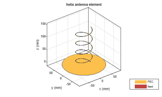
Create and view a helix antenna that has a 28 mm turn radius, 1.2 mm strip width, and 4 turns.

hx = helix(Radius=28e-3, Width=1.2e-3, Turns=4)

hx = 
  helix with properties:

               Radius: 0.0280
                Width: 0.0012
                Turns: 4
              Spacing: 0.0350
     WindingDirection: 'CCW'
       FeedStubHeight: 1.0000e-03
    GroundPlaneRadius: 0.0750
            Substrate: [1×1 dielectric]
            Conductor: [1×1 metal]
                 Tilt: 0
             TiltAxis: [1 0 0]
                 Load: [1×1 lumpedElement]

show(hx)

Radiation Pattern of Helix Antenna

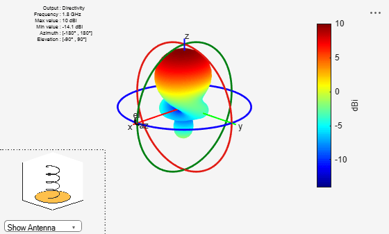
Plot the radiation pattern of a helix antenna.

hx = helix(Radius=28e-3,Width=1.2e-3,Turns=4);
pattern(hx,1.8e9);

Calculate Spacing of Helix Antenna with Varying Radius

Calculate the spacing of a helix that has a pitch of 12 degrees and a radius that varies from 20 mm to 22 mm in steps of 0.5 mm.

s = helixpitch2spacing(12,20e-3:0.5e-3:22e-3)

s = 1×5

    0.0267    0.0274    0.0280    0.0287    0.0294

Radiation Pattern of Helix Antenna

Plot the radiation pattern of a helix antenna with transparency specified as 0.5.

p = PatternPlotOptions

p = 
  PatternPlotOptions with properties:

      Transparency: 1
         SizeRatio: 0.9000
    MagnitudeScale: []
     AntennaOffset: [0 0 0]

p.Transparency = 0.5;
ant = helix;
pattern(ant,2e9,patternOptions=p)

To understand the effect of Transparency, chose Overlay Antenna in the radiation pattern plot.

This option overlays the helix antenna on the radiation pattern.

Helix Antenna with Dielectric Substrate

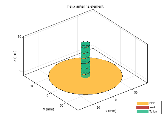
Create a custom helix antenna with a Teflon dielectric substrate.

d = dielectric("Teflon"); 
hx = helix(Width=0.815e-3, Turns=6, Radius=9.3e-3, Spacing=12.4e-3, Substrate=d)

hx = 
  helix with properties:

               Radius: 0.0093
                Width: 8.1500e-04
                Turns: 6
              Spacing: 0.0124
     WindingDirection: 'CCW'
       FeedStubHeight: 1.0000e-03
    GroundPlaneRadius: 0.0750
            Substrate: [1×1 dielectric]
            Conductor: [1×1 metal]
                 Tilt: 0
             TiltAxis: [1 0 0]
                 Load: [1×1 lumpedElement]

View the helix antenna.

show(hx)

References

[1] Balanis, C.A. Antenna Theory. Analysis and Design, 3rd Ed. New York: Wiley, 2005.

[2] Volakis, John. Antenna Engineering Handbook, 4th Ed. New York: Mcgraw-Hill, 2007.

[3] Zhang, Yan, Q. Ding, J. Chen, S. Lu, Z. Zhu and L. L. Cheng. “A Parametric Study of Helix Antenna for S-Band Satellite Communications.” 9th International Symposium on Antenna Propagation and EM Theory (ISAPE). 2010, pp. 193–196.

[4] Djordjevic, A.R., Zajic, A.G., Ilic, M. M., Stuber, G.L. “Optimization of Helical antennas (Antenna Designer's Notebook)” IEEE Antennas and Propagation Magazine. December, 2006, pp. 107, pp.115.

[5] B. Young, K. A. O'Connor and R. D. Curry, “Reducing the size of helical antennas by means of dielectric loading,” 2011 IEEE Pulsed Power Conference, 2011, pp. 575-579, doi: 10.1109/PPC.2011.6191490

Version History

Introduced in R2015a