Room Impulse Response Simulation with the Image-Source Method and HRTF Interpolation
Room impulse response simulation aims to model the reverberant properties of a space without having to perform acoustic measurements. Many geometric and wave-based room acoustic simulation methods exist in the literature [1]. The image-source method is a popular and relatively straightforward geometric method [2]. It models the specular reflections between a transmitter and a receiver.
Image-source is a geometric simulation method that models specular sound reflection paths between the source and receiver. It assumes that sound travels in straight lines (rays) which undergo perfect reflections when they encounter an obstacle (in our case, one of the four walls, the floor, or the ceiling of the room).
When a sound ray hits a wall, it spawns a mirrored "image" source. The image source is the symmetrical reflection of the original source with respect to the encountered boundary. Higher-order reflections (rays that reach the receiver after bouncing off multiple obstacles) are modeled by repeating the mirroring process with respect to each encountered obstacle.
First, this example shows how to use acousticRoomResponse to apply image-source in one line of code. Then, the example showcases the image-source method step by step for a simple "shoebox" (cuboid) room. The example also uses head-related transfer function (HRTF) interpolation to simulate the received sound at the ears of the listener.
Use acousticRoomResponse to Perform Image-Source
Synthesize Impulse Response of Shoebox Room
Start with performing image-source on a shoebox room.
Define Room Parameters
Define the room dimensions, in meters (width, length and height, respectively).
roomDimensions = [4 4 2.5];
You treat the receiver and transmitter as points within the space of the room. Define their coordinates, in meters.
rx = [2 1 1.8];
tx = [3 1 1.8];
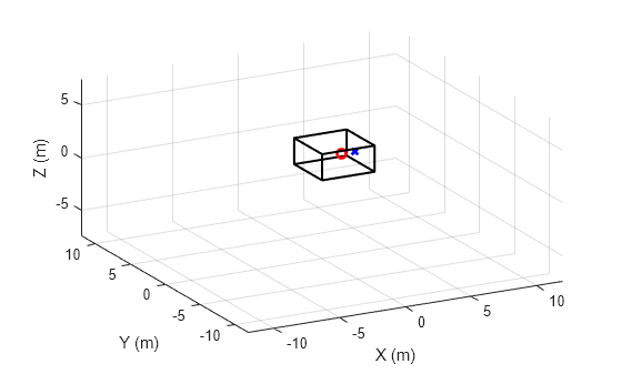
Plot the room space along with the receiver (red circle) and transmitter (blue x).
h = figure;
plotRoom(roomDimensions,rx,tx,h)

Define Wall Absorption Coefficients
Define the absorption coefficients of the walls. The absorption coefficient is a measure of how much sound is absorbed (rather than reflected) when hitting a surface.
The absorption coefficients are frequency-dependent and are defined at the frequencies defined in the variable FVect [4]. Each row represents the coefficients of a wall (floor, front wall, back wall, left wall, right wall, and ceiling).
FVect = [125 250 500 1000 2000 4000];

A = [0.10 0.20 0.40 0.60 0.50 0.60;...
    0.10 0.20 0.40 0.60 0.50 0.60;...
    0.10 0.20 0.40 0.60 0.50 0.60;...
    0.10 0.20 0.40 0.60 0.50 0.60;...
    0.02 0.03 0.03 0.03 0.04 0.07;...
    0.02 0.03 0.03 0.03 0.04 0.07].';
Synthesize Impulse Response
Synthesize and plot the impulse response. Specify the algorithm as "image-source". Specify an image-source order of 5. This defines the maximum number of reflections.
Use a sampling rate of 44.1 kHz.
fs = 44.1e3;
ir = acousticRoomResponse(roomDimensions,tx,rx,...
                          SampleRate=fs,...
                          Algorithm="image-source",...
                          ImageSourceOrder=5,...
                          BandCenterFrequencies=FVect,...
                          AirAbsorption=0,...
                          MaterialAbsorption=A.');

figure
plot((1/fs)*(0:numel(ir)-1),ir)
grid on
xlabel("Time (s)")
ylabel("Impulse Response")

Auralization
Apply the impulse response to an audio signal.
Load an audio signal.
[audioIn,fs] = audioread("FunkyDrums-44p1-stereo-25secs.mp3");
audioIn = audioIn(:,1);
Listen to a few seconds of the original audio.
T = 10;
sound(audioIn(1:T*fs),fs)
pause(T)
Simulate the received audio by filtering with the impulse response.
audioOut = filter(ir,1,audioIn);
audioOut = audioOut/max(audioOut);
Listen to a few seconds of the received audio.
sound(audioOut(1:T*fs),fs)
pause(T)
Synthesize Impulse Response of Non-Shoebox Room
Synthesize the impulse response of a more complex, non-shoebox room.
3-D model information is often stored in stereolithography (STL) files.
Load the room setup from a sample STL file.
room = stlread("room.stl");Visualize the room along with the source and receiver positions. Notice that the room includes a partition wall. In this example, there is no line-of-sight between the transmitter and the receiver.
tx = [1 1 1.8];
rx = [3.5 3 1.7];
figure
visualizeGeneralRoom(room,tx,rx)

Synthesize the impulse response.
ir = acousticRoomResponse(room,tx,rx,SampleRate=fs,Algorithm="image-source",ImageSourceOrder=5);

figure
plot((1/fs)*(0:numel(ir)-1),ir)
grid on
xlabel("Time (s)")
ylabel("Impulse Response")

Simulate the received audio by filtering with the impulse response.
audioOut = filter(ir,1,audioIn);
audioOut = audioOut/max(audioOut);
Listen to a few seconds of the received audio.
sound(audioOut(1:T*fs),fs)
pause(T)
Construct Room with Triangulation Objects
In the previous section, you loaded the room from an STL file.
You can also construct a custom room with triangulation objects. You can assign different custom material characteristics to each wall or section of the room.
Start with the room exterior.
roomDimensions = [5 4 6];

X = roomDimensions(1);
Y = roomDimensions(2);
Z = roomDimensions(3);

pts = [0 0 0;
       X 0 0;
       0 Y 0;
       X Y 0;
       0 0 Z;
       0 Y Z;
       X 0 Z;
       X Y Z];

dt = delaunayTriangulation(pts(:,1), pts(:,2), pts(:,3));
[conn, verts] = freeBoundary(dt);
Define the absorption coefficients of the room. Use the same coefficients for all the walls in the room.
roomAbsorption = repmat([0.02 0.02 0.03 0.03 0.04 0.05 0.05],12,1);
Next, design a partition wall in the room.
wallDimensions = [4 .2 4.5];

X = wallDimensions(1);
Y = wallDimensions(2);
Z = wallDimensions(3);

pts = [0 0 0;
       X 0 0;
       0 Y 0;
       X Y 0;
       0 0 Z;
       0 Y Z;
       X 0 Z;
       X Y Z] + [0 2 0];

dt2 = delaunayTriangulation(pts(:,1), pts(:,2), pts(:,3));
[conn2, verts2] = freeBoundary(dt2);
conn2 = conn2 + size(verts,1);
Define the absorption coefficients of the wall.
wallAbsorption = repmat([0.02 0.03 0.04 0.05 0.04 0.03 0.02],12,1);
Combine the room and the partition wall.
room = triangulation([conn;conn2],[verts;verts2])
room =
  triangulation with properties:

              Points: [16×3 double]
    ConnectivityList: [24×3 double]
Visualize the room using the helper function visualizeGeneralRoom.
visualizeGeneralRoom(room,tx,rx)

Combine the absorption coefficients of the room and the partition wall.
roomAbsorption = [roomAbsorption;wallAbsorption];
Synthesize and plot the impulse response of the room.
ir = acousticRoomResponse(room,tx,rx,...
                         Algorithm="image-source",...
                         BandCenterFrequencies=[125 250 500 1000 2000 4000 8000],...
                         MaterialAbsorption=roomAbsorption);
t = (0:numel(ir)-1)/fs;
figure
plot(t,ir)
grid on
xlabel("Time (s)")
ylabel("Impulse Response")

Simulate the received audio by filtering with the impulse response.
audioOut = filter(ir,1,audioIn);
audioOut = audioOut/max(audioOut);
Listen to a few seconds of the received audio.
sound(audioOut(1:T*fs),fs)
The Image-Source Method
In this section, you learn how acousticRoomResponse operates by implementing the image-source algorithm step-by-step. For simplicity, you use a simple shoebox room.
Define Room Parameters
Define the room dimensions, in meters (width, length and height, respectively).
roomDimensions = [4 4 2.5];
You treat the receiver and transmitter as points within the space of the room. Define their coordinates, in meters.
rx = [2 1 1.8];
tx = [3 1 1.8];
Plot the room space along with the receiver (red circle) and transmitter (blue x).
h = figure;
plotRoom(roomDimensions,rx,tx,h)

Visualize One Image
Recall that in the image-source method, when a sound ray hits a wall, it spawns a mirrored "image" source. The image source is the symmetrical reflection of the original source with respect to the encountered boundary. Higher-order reflections (rays that reach the receiver after bouncing off multiple obstacles) are modeled by repeating the mirroring process with respect to each encountered obstacle.
As an example, consider the ray that bounces off two walls and the floor before arriving at the receiver. Define the coordinates of the equivalent image for this ray.
imageSource = [-tx(1) -tx(2) -tx(3)];
The ray is modeled by the straight line connecting the image to the receiver. The length of this straight line is equal to the traveled distance from the original source to the receiver along the reflected ray.
Visualize the image-source and the resulting path.
plot3(imageSource(1),imageSource(2),imageSource(3),"gx",LineWidth=2)
plot3([imageSource(1) rx(1)], ...
      [imageSource(2) rx(2)], ...
      [imageSource(3) rx(3)],Color="k",LineWidth=2)

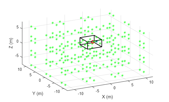
Visualize Multiple Images
To calculate the room impulse response, add the contributions of a large number of source images.
Extend the visible space around the room to ensure the images appear in the plot.
h2 = figure;

plotRoom(roomDimensions,rx,tx,h2)

Lx = roomDimensions(1);
Ly = roomDimensions(2);
Lz = roomDimensions(3);

xlim([-3*Lx,3*Lx]);
ylim([-3*Ly,3*Ly]);
zlim([-3*Lz,3*Lz]);
Visualize a subset of the source images. Compute the image coordinates based on equations 6 and 7 in [2].
Model the eight combinations stemming from possible reflections along the x-, y- and z- axes.
x = tx(1);
y = tx(2);
z = tx(3);
sourceXYZ = [-x -y -z;...
             -x -y  z;...
             -x  y -z;...
             -x  y  z;...
              x -y -z;...
              x -y  z;...
              x  y -z;...
              x  y  z].';
Model scenarios with multiple reflections by looping over the x-, y- and z- axes. These loops have infinite ranges in theory. You will see how to practically limit the ranges in the next section. For now, select arbitrary limits for the loops.
% Increase the range to plot more images
nVect = -2:2;
lVect = -2:2;
mVect = -2:2;

for n = nVect
    for l = lVect
        for m = mVect
            xyz = [n*2*Lx; l*2*Ly; m*2*Lz];
            isourceCoords = xyz - sourceXYZ;
            for kk=1:8
                isourceCoord=isourceCoords(:,kk);
                plot3(isourceCoord(1),isourceCoord(2),isourceCoord(3),"g*")
            end
        end
    end
end
Restrict the Number of Simulated Images
The number of images is theoretically infinite. Restrict the number of images by limiting the computed impulse response length to the time by which the reverberated sound pressure drops below a certain level. Here, you use the reverberation time RT60 [3], which is the time by which the sound level has dropped by 60 dB.
You use Sabine's formula to calculate RT60.
Define Wall Absorption Coefficients
First, define the absorption coefficients of the walls at the frequencies defined in the variable FVect [4].
FVect = [125 250 500 1000 2000 4000];

A = [0.10 0.20 0.40 0.60 0.50 0.60;...
    0.10 0.20 0.40 0.60 0.50 0.60;...
    0.10 0.20 0.40 0.60 0.50 0.60;...
    0.10 0.20 0.40 0.60 0.50 0.60;...
    0.02 0.03 0.03 0.03 0.04 0.07;...
    0.02 0.03 0.03 0.03 0.04 0.07].';
Estimate RT60
Compute RT60 based on Sabine's formula.
First, compute the room's volume.
V = Lx*Ly*Lz;
Next, compute the total wall surface area of the room.
WallXZ = Lx*Lz;
WallYZ = Ly*Lz;
WallXY = Lx*Ly;
Compute the frequency-dependent effective absorbing area of the room surfaces.
S = WallYZ*(A(:,1)+A(:,2))+WallXZ.*(A(:,3)+A(:,4))+WallXY.*(A(:,5)+A(:,6));
Compute the frequency-dependent RT60, in seconds, based on Sabine's equation. Notice that RT60 is frequency-dependent: There are 6 different RT60 values, one for each frequency band.
c  = 343; % Speed of sound (m/s)
RT60 = (55.25/c)*V./S
RT60 = 6×1
1.3886
0.7191
0.3799
0.2581
0.3028
0.2455
Deduce the maximum impulse response length (in samples) based on the largest value in RT60.
impResLength = fix(max(RT60)*fs)
impResLength =
61237
Express the maximum range of the impulse response in meters.
impResRange=c*(1/fs)*impResLength
impResRange =
476.2878
Use this value to limit the range over which to compute images. In this example, to limit the run time, you restrict the loop ranges to [-10;10].
nMax = min(ceil(impResRange./(2.*Lx)),10);
lMax = min(ceil(impResRange./(2.*Ly)),10);
mMax = min(ceil(impResRange./(2.*Lz)),10);
Derive Contribution of One Image
In this section, you derive the contribution of one image to the room impulse response.
You later obtain the full room impulse response by summing the contributions of all images under consideration.
Derive the pressure reflection coefficients from the absorption coefficients.
B=sqrt(1-A);
Store the reflection coefficients for each wall in a separate variable.
BX1=B(:,1);
BX2=B(:,2);
BY1=B(:,3);
BY2=B(:,4);
BZ1=B(:,5);
BZ2=B(:,6);
Model the eight permutations representing the absence or presence of reflection on the x-, y-, and z- axes.
surface_coeff=[0 0 0; 0 0 1; 0 1 0; 0 1 1; 1 0 0; 1 0 1; 1 1 0; 1 1 1];
q = surface_coeff(:,1).';
j = surface_coeff(:,2).';
k = surface_coeff(:,3).';
In this section, you focus on the contribution of a single image. Select index values corresponding to an arbitrary image.
n = 1;
l = 1;
m = 1;
p = 1;
Compute Image Delay
The contribution of each image is defined by two values:
Delay: The time it takes the signal to reach the receiver.
Power: The (frequency-dependent) energy level of the signal when it reaches the receiver.
You start by computing the image delay. The delay is related to the total distance traveled by the wave from the image to the receiver.
Get the coordinates of the image.
isourceCoord = [n*2*Lx; l*2*Ly; m*2*Lz] - sourceXYZ(:,p);
Calculate the delay (in samples) at which the contribution occurs.
dist = norm((isourceCoord(:)-rx(:)),2);
delay = (fs/c).*dist;
Compute Image Power
Now compute the frequency-dependent magnitude of the contribution.
ImagePower = BX1.^abs(n-q(p)).*BY1.^abs(l-j(p)).*BZ1.^abs(m-k(p)).*BX2.^abs(n).*(BY2.^abs(l)).*(BZ2.^abs(m));
Derive Image Contribution
The image power is only defined at 6 frequencies. Here, you first interpolate the response to the entire frequency (Nyquist) range, and then perform an inverse FFT operation to derive the image's contribution to the impulse response.
Extend the energy level to incorporate zero and Nyquist frequencies.
FVect2=[0 FVect fs/2]';
ImagePower2 = [ImagePower(1); ImagePower(:); ImagePower(6)];
In this example, use an FFT length of 512.
FFTLength = 512;
HalfLength = fix(FFTLength./2);
OneSidedLength = HalfLength+1;
Interpolate the response to the entire frequency range.
ImagePower2 = interp1(FVect2./(fs/2),ImagePower2,linspace(0,1,257)).';
Convert the response to two-sided.
ImagePower2 = [ImagePower2; conj(ImagePower2(HalfLength:-1:2))];
Convert the frequency response to the time-based contribution of the image.
h_ImagePower = real(ifft(ImagePower2,FFTLength));
Smooth the response by applying a Hann window.
win = hann(FFTLength+1);
h_ImagePower = win.*[h_ImagePower(OneSidedLength:FFTLength); ...
                     h_ImagePower(1:OneSidedLength)];
HRTF Modeling
You have derived the image's contribution to the impulse response, where you assumed that the receiver is a point in space. Here, you derive the image's contribution at the ears of a listener located at the receiver coordinates by using 3-D head-related transfer function (HRTF) interpolation.
You use the ARI HRTF data set [5]. Load the data set.
ARIDataset = load("ReferenceHRTF.mat");Express the hrtfData as an array of size (Number of source measurements) × 2 × (Sample lengths).
hrtfData = permute(ARIDataset.hrtfData,[2 3 1]);
sourcePosition = ARIDataset.sourcePosition(:,[1 2]);

Calculate the elevation and azimuth corresponding to the coordinates of the image source.
sensor_xyz=rx;
xyz=isourceCoord-sensor_xyz;
hyp = sqrt(xyz(1)^2+xyz(2)^2);
elevation = atan(xyz(3)./(hyp+eps));
azimuth = atan2(xyz(2),xyz(1));
The desired HRTF position is formed by the computed elevation and azimuth.
desiredPosition = [azimuth elevation]*180/pi;
Calculate the HRTF at the desired position.
interpolatedIR  = interpolateHRTF(hrtfData,sourcePosition,desiredPosition);
interpolatedIR = squeeze(permute(interpolatedIR,[3 2 1]));
Incorporate the HRTF into the response using convolution.
interpolatedIR = [interpolatedIR; zeros(512,2)];
h = [];
h(:,1) = filter(h_ImagePower,1,interpolatedIR(:,1));
h(:,2) = filter(h_ImagePower,1,interpolatedIR(:,2));
Plot the overall contribution of the selected image. This contribution is added to the overall impulse response at the computed image delay.
figure
plot(1:size(h,1),h)
grid on
xlabel("Sample Index")
ylabel("Impulse Response")
legend("Left","Right")

Compute the Impulse Response
In this section, you compute the overall impulse response by summing the contributions of individual images. The contribution of each image is computed exactly like in the previous section.
The helper function HelperImageSource encapsulates the steps you went over in the previous section. It computes the impulse response by summing image contributions.
useHRTF = true;
h = HelperImageSource(roomDimensions,rx,tx,A,FVect,fs,useHRTF,hrtfData,sourcePosition);
Visualize Impulse Response
Plot the impulse response.
figure
t= (1/fs)*(0:size(h,1)-1);
plot(t,h)
grid on
xlabel("Time (s)")
ylabel("Impulse Response")
legend("Left","Right")

Auralization
Apply the impulse response to an audio signal.
Load an audio signal.
[audioIn,fs] = audioread("FunkyDrums-44p1-stereo-25secs.mp3");
audioIn = audioIn(:,1);
Simulate the received audio by filtering with the impulse response.
y1 = filter(h(:,1),1,audioIn);
y2 = filter(h(:,2),1,audioIn);
y = [y1 y2];
Listen to a few seconds of the original audio.
T = 10;
sound(audioIn(1:fs*T),fs)
pause(T)
Listen to a few seconds of the received audio.
sound(y(1:fs*T),fs);
References
[1] Savioja, Lauri, and U. Peter Svensson. “Overview of Geometrical Room Acoustic Modeling Techniques.” The Journal of the Acoustical Society of America 138, no. 2 (2015): 708–30. https://doi.org/10.1121/1.4926438.
[2] Allen, Jont B., and David A. Berkley. “Image Method for Efficiently Simulating Small-Room Acoustics.” The Journal of the Acoustical Society of America 65, no. 4 (1979): 943–50. https://doi.org/10.1121/1.382599.
[3] "Sabine’s Formula & The Birth of Modern Architectural Acoustics", accessed Sept. 5, 2025, https://www.thermaxxjackets.com/news/sabine-modern-architectural/.
[4] Absorption coefficients, accessed Sept. 5, 2025, https://www.acoustic.ua/st/web_absorption_data_eng.pdf.
[5] ARI HRTF Database at the Acoustic Research Institute of the Austrian Academy of Sciences, accessed Sept. 5, 2025, https://www.oeaw.ac.at/isf/outreach/software/hrtf-database.
Helper Functions
function plotRoom(roomDimensions,receiverCoord,sourceCoord,figHandle)
% PLOTROOM Plot room, transmitter and receiver

figure(figHandle)
X = [0;roomDimensions(1);roomDimensions(1);0;0];
Y = [0;0;roomDimensions(2);roomDimensions(2);0];
Z = [0;0;0;0;0];
figure;
hold on;
plot3(X,Y,Z,"k","LineWidth",1.5);   % draw a square in the xy plane with z = 0
plot3(X,Y,Z+roomDimensions(3),"k","LineWidth",1.5); % draw a square in the xy plane with z = 1
set(gca,"View",[-28,35]); % set the azimuth and elevation of the plot
for k=1:length(X)-1
    plot3([X(k);X(k)],[Y(k);Y(k)],[0;roomDimensions(3)],"k","LineWidth",1.5);
end
grid on
xlabel("X (m)")
ylabel("Y (m)")
zlabel("Z (m)")
plot3(sourceCoord(1),sourceCoord(2),sourceCoord(3),"bx","LineWidth",2)
plot3(receiverCoord(1),receiverCoord(2),receiverCoord(3),"ro","LineWidth",2)
end

function h = HelperImageSource(roomDimensions,receiverCoord, ....
                    sourceCoord,A,FVect,fs,useHRTF,varargin)
% HELPERIMAGESOURCE Estimate impulse response of shoebox room
% roomDimensions: Room dimensions, specified as a row vector with three
%                 values.
% receiverCoord: Receiver coordinates, specified as a row vector with 3
%                values
% sourceCoord: Source coordinates, specified as a row vector with 3
%              values
% A:  Wall absorption coefficient matrix, specified as a L-by-6 matrix,
%     where L is the number of frequency bands.
% FVect: Vector of frequencies, of length L.
% fs: Sampling rate, in Hertz
% useHRTF: Specify as true to use HRTF interpolation
% hrtfData: Specify is useHRTF is true
%sourcePosition: Specify is useHRTF is true

hrtfData = [];
sourcePosition = [];
if useHRTF
    hrtfData = varargin{1};
    sourcePosition = varargin{2};
end

x = sourceCoord(1);
y = sourceCoord(2);
z = sourceCoord(3);
sourceXYZ = [-x -y -z; ...
             -x -y  z; ...
             -x  y -z; ...
             -x  y  z; ...
              x -y -z; ...
              x -y  z; ...
              x  y -z; ...
              x  y  z].';

Lx=roomDimensions(1);
Ly=roomDimensions(2);
Lz=roomDimensions(3);

V = Lx*Ly*Lz;

WallXZ=Lx*Lz;
WallYZ=Ly*Lz;
WallXY=Lx*Ly;

S = WallYZ*(A(:,1)+A(:,2))+WallXZ.*(A(:,3)+A(:,4))+WallXY.*(A(:,5)+A(:,6));

c  = 343; % Speed of sound (m/s)
RT60 = (55.25/c)*V./S;

impResLength = fix(max(RT60)*fs);

impResRange=c*(1/fs)*impResLength;

nMax = min(ceil(impResRange./(2.*Lx)),10);
lMax = min(ceil(impResRange./(2.*Ly)),10);
mMax = min(ceil(impResRange./(2.*Lz)),10);

B=sqrt(1-A);

BX1=B(:,1);
BX2=B(:,2);
BY1=B(:,3);
BY2=B(:,4);
BZ1=B(:,5);
BZ2=B(:,6);

surface_coeff=[0 0 0; 0 0 1; 0 1 0; 0 1 1; 1 0 0; 1 0 1; 1 1 0; 1 1 1];
q=surface_coeff(:,1).';
j=surface_coeff(:,2).';
k=surface_coeff(:,3).';

FFTLength=512;
HalfLength=fix(FFTLength./2);
OneSidedLength = HalfLength+1;
win = hann(FFTLength+1);

FVect2=[0 FVect fs/2]';

h = zeros(impResLength,2);

for n=-nMax:nMax
    Lxn2=n*2*Lx;
    for l=-lMax:lMax
        Lyl2=l*2*Ly;

       if useHRTF
            imagesVals = zeros(FFTLength+size(hrtfData,3),2,2*lMax+1,8);
       else
           imagesVals = zeros(FFTLength+1,2,2*lMax+1,8);
       end

        Li = size(imagesVals,1);
        isDelayValid = zeros(2*lMax+1,8);
        start_index_HpV = zeros(2*lMax+1,8);
        stop_index_HpV = zeros(2*lMax+1,8);
        start_index_hV = zeros(2*lMax+1,8);

        parfor mInd=1:2*mMax+1

            m = mInd - mMax - 1;

            Lzm2=m*2*Lz;
            xyz = [Lxn2; Lyl2; Lzm2];

            isourceCoordV=xyz - sourceXYZ;
            xyzV = isourceCoordV - receiverCoord.';
            distV = sqrt(sum(xyzV.^2));
            delayV = (fs/c)*distV;

            ImagePower = BX1.^abs(n-q).*BY1.^abs(l-j).*BZ1.^abs(m-k).*BX2.^abs(n).*(BY2.^abs(l)).*(BZ2.^abs(m));
            ImagePower2 = [ImagePower(1,:); ImagePower; ImagePower(6,:)];

            ImagePower2 = ImagePower2./distV;

            validDelay = delayV<= impResLength;

            if sum(validDelay)==0
                continue;
            end

            isDelayValid(mInd,:) = validDelay;

            ImagePower2 = interp1(FVect2./(fs/2),ImagePower2,linspace(0,1,257));
            if isrow(ImagePower2)
                ImagePower2 = ImagePower2.';
            end
            ImagePower3 = [ImagePower2; conj(ImagePower2(HalfLength:-1:2,:))];

            h_ImagePower = real(ifft(ImagePower3,FFTLength));
            h_ImagePower = [h_ImagePower(OneSidedLength:FFTLength,:); h_ImagePower(1:OneSidedLength,:)];
            h_ImagePower = win.*h_ImagePower;

            if useHRTF
                hyp = sqrt(xyzV(1,:).^2+xyzV(2,:).^2);
                elevation = atan(xyzV(3,:)./(hyp+realmin));
                azimuth = atan2(xyzV(2,:),xyzV(1,:));

                desiredPosition = [azimuth.',elevation.']*180/pi;

                interpolatedIR  = interpolateHRTF(hrtfData,sourcePosition,desiredPosition,"Algorithm","VBAP");
                interpolatedIR = squeeze(permute(interpolatedIR,[3 2 1]));

                pad_ImagePower = zeros(512,2);

                for index=1:8
                    hrir0 = interpolatedIR(:,:,index);
                    hrir_ext=[hrir0; pad_ImagePower];
                    for ear=1:2
                        imagesVals(:,ear,mInd,index)=filter(h_ImagePower(:,index),1,hrir_ext(:,ear));
                    end
                end
            else
                for index=1:8
                    for ear=1:2
                        imagesVals(:,ear,mInd,index)=h_ImagePower(:,index);
                    end
                end
            end

            adjust_delay = round(delayV) - (fix(FFTLength/2))+1;

            len_h=Li;
            start_index_HpV(mInd,:) = max(adjust_delay+1+(adjust_delay>=0),1);
            stop_index_HpV(mInd,:) = min(adjust_delay+1+len_h,impResLength);
            start_index_hV(mInd,:) = max(-adjust_delay,1);

        end
        stop_index_hV = start_index_hV + (stop_index_HpV - start_index_HpV);

        for index2=1:size(imagesVals,3)
            for index3=1:8
                if isDelayValid(index2,index3)
                    h(start_index_HpV(index2,index3):stop_index_HpV(index2,index3),:)= h(start_index_HpV(index2,index3):stop_index_HpV(index2,index3),:) + squeeze(imagesVals(start_index_hV(index2,index3):stop_index_hV(index2,index3),:,index2,index3));
                end
            end
        end

    end
end

h = h./max(abs(h));
end

function visualizeGeneralRoom(tri,SourceCoordinates,ReceiverCoordinates)
figure;
trisurf(tri, ...
    'FaceAlpha', 0.3, ...
    'FaceColor', [.5 .5 .5], ...
    'EdgeColor', 'none');
view(60, 30);
hold on; axis equal; grid off;
xlabel('x'); ylabel('y'); zlabel('z');
% Plot edges
fe = featureEdges(tri,pi/20);
numEdges = size(fe, 1);
pts = tri.Points;
a = pts(fe(:,1),:);
b = pts(fe(:,2),:);
fePts = cat(1, reshape(a, 1, numEdges, 3), ...
           reshape(b, 1, numEdges, 3), ...
           nan(1, numEdges, 3));
fePts = reshape(fePts, [], 3);
plot3(fePts(:, 1), fePts(:, 2), fePts(:, 3), 'k', 'LineWidth', .5);

hold on
sourceCoord = SourceCoordinates;
receiverCoord = ReceiverCoordinates;
scatter3(sourceCoord(1), sourceCoord(2), sourceCoord(3), 'sb', 'filled');
scatter3(receiverCoord(1,1), receiverCoord(1,2), receiverCoord(1,3), 'sr', 'filled');
end