samplealign
Align peaks in signal to reference peaks
Description
Examples
Create two signals with noisy Gaussian peaks.
rng('default')
peakLoc = [30 60 90 130 150 200 230 300 380 430];
peakInt = [7 1 3 10 3 6 1 8 3 10];
time = 1:450;
comp = exp(-(bsxfun(@minus,time,peakLoc')./5).^2);
sig_1 = (peakInt + rand(1,10)) * comp + rand(1,450);
sig_2 = (peakInt + rand(1,10)) * comp + rand(1,450);
Define a nonlinear warping function.
wf = @(t) 1 + (t<=100).*0.01.*(t.^2) + (t>100).*...
     (310+150*tanh(t./100-3));
Warp the second signal to distort it.
sig_2 = interp1(time,sig_2,wf(time),'pchip');Align the observations between the two signals by introducing gaps.
[i,j] = samplealign([time;sig_1]',[time;sig_2]',...
                    'weights',[0,1],'band',35,'quantile',.5);
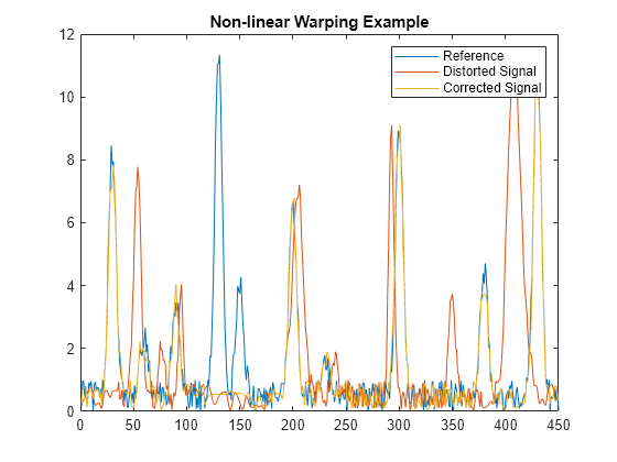
Plot the reference signal, distorted signal, and warped (corrected) signal.
figure
sig_3 = interp1(time,sig_2,interp1(i,j,time,'pchip'),'pchip');
plot(time,sig_1,time,sig_2,time,sig_3)
legend('Reference','Distorted Signal','Corrected Signal')
title('Non-linear Warping Example')

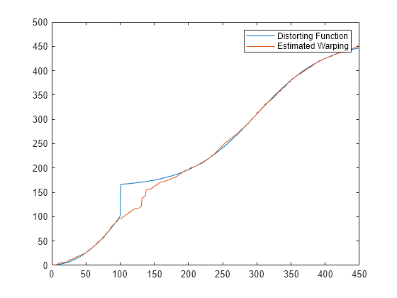
Plot the real and the estimated warping functions.
figure
plot(time,wf(time),time,interp1(j,i,time,'pchip'))
legend('Distorting Function','Estimated Warping')

Input Arguments
Data containing sequential observations, specified as a real matrix. Rows
of X correspond to observations or samples, and columns
correspond to features or dimensions. The first column is the
reference dimension, and must contain unique
values in ascending order. The reference dimension could contain sample
indices of the observations or a measurable value, such as time.
Data Types: double
Data containing sequential observations, specified as a real matrix. Rows
of Y correspond to observations or samples, and columns
correspond to features or dimensions. The first column is the reference
dimension and must contain unique values in ascending order. The reference
dimension could contain sample indices of the observations or a measurable
value, such as time.
Data Types: double
Name-Value Arguments
Specify optional pairs of arguments as
Name1=Value1,...,NameN=ValueN, where Name is
the argument name and Value is the corresponding value.
Name-value arguments must appear after other arguments, but the order of the
pairs does not matter.
Example: samplealign(X,Y,ShowNetwork=true) plots the resulting
dynamic programming statistics after computing the alignment
Maximum allowable distance between observations along the reference
dimension, specified as a positive scalar, Inf, or a
function handle.
Band limits the number of potential matches between
observations in two data sets. If S is the value in
the reference dimension for a given observation (row) in one data set,
then that observation is matched only with observations in the other
data set whose values in the reference dimension fall within
S ± Band. Only these
potential matches are passed to the algorithm for further
scoring.
If you specify Band as a function handle,
samplealign sequentially passes the midpoint
between each of the reference observations (scalars)
x(i) in one data set and a given reference
observation y(j) in the other data set.
samplealign checks whether
|x(i) – y(j)| ≤
band((x(i) +
y(j))/2)
and if so, the observations X(i,:) and
Y(j,:) are potential matches.
The Band constraint reduces the time and memory
complexity of the algorithm from O(MN) to
O(sqrt(MN)*K), where
M and N are the number of
observations in X and Y
respectively, and K is a small constant such that
K<<M and
K<<N. Adjust
Band to the maximum expected shift between the
reference dimensions in the two data sets, that is, between
X(:,1) and Y(:,1).
Note
If you specify both Band and Width, only pairs of observations that meet both constraints are considered potential matches and passed to the algorithm for scoring.
Tip
Specify Width when you do not have a good estimate for Band. To get an indication of the memory required to run the algorithm with specific Band and Width parameters on your data sets, run samplealign, but do not specify return values and set ShowConstraints to true.
Example: 15
Data Types: double | function_handle
Function to calculate distance between pairs of observations that are
potential matches, specified as a function handle of the form
@(r,s)function(r,s). The function accepts
r and s as matrices of the
same size whose paired rows represent all potential matches of
observations in X and Y
respectively. The function returns a column vector of nonnegative
distance values with the same number of rows as r and
s.
Distance uses all columns in X
and Y, including the reference dimension, when
calculating distances. If you do not want to include the reference
dimension in the distance calculations, use the
Weights name-value argument to exclude
it.
Data Types: function_handle
Penalty for an observation being matched to a gap in the other data set, specified as one of the following.
Cell array of two function handles,
{@(x)G(x),@(y)H(y)}. Each of the functionsGandHcalculate the penalty for an observation (row) when it is matched to a gap in the other data set. These functions return a column vector of penalty values with the same number of rows asXorY.Single function handle
@(x)Z(x)usesZas both functions in the cell array syntax:{@(x)Z(x),@(y)Z(y)}.The two-element cell array can contain a scalar value instead of a function handle for either or both entries. In this case, the scalar value is used as the penalty for a row being matched to gap.
A single nonnegative scalar value is used as the penalty for all rows matched to a gap.
Gap specifies the position-dependent terms for
assigning gap penalties. The calculated value, GPX,
is the gap penalty for matching observations from the first data set
X to gaps inserted in the second data set
Y, and is the product of two terms:
GPX = G *
QMS. The term G takes its
value as a function of the observations in X.
Similarly, GPY is the gap penalty for matching
observations from Y to gaps inserted in
X, and is the product of two terms:
GPY = H *
QMS. The term H takes its
value as a function of the observations in Y. By
default, the term QMS is the 0.75 quantile of the
score for the pairs of observations that are potential matches (that is,
pairs that comply with the Band and
Width constraints).
Note
Gap defaults to a relatively safe value.
However, the success of the algorithm depends on the fine tuning of
the gap penalties, which is application dependent. When the gap
penalties are large relative to the score of the correct matches,
samplealign returns alignments with fewer
gaps, but with more incorrectly aligned regions. When the gap
penalties are smaller, the output alignment contains longer regions
with gaps and fewer matched observations. Set
ShowNetwork to true to
compare the gap penalties to the score of matched observations in
different regions of the alignment.
Example: 10
Data Types: double | cell | function_handle
Quantile value used to calculate QMS for
Gap, a scalar between 0 and
1.
Example: 0.5
Data Types: double
Indication to plot sample matching, specified as
false (do not plot), true
(plot the data for column 2), or a positive integer that is the index of
the column of data to plot. The plot uses the reference dimension as the
horizontal axis, the selected index as the vertical axis, and shows
links between all the potential matches that meet the constraints, the
potential and selected matches along with the data from
X and Y.
See Algorithms.
Example: true
Data Types: logical
Indication to plot Band and
Width data, specified as false
(do not plot) or true (plot the data). Use the plot
to estimate the memory required to run the algorithm with specific
'Band' and 'Width' on your
data set.
See Algorithms.
Example: true
Data Types: logical
Indication to plot dynamic programming statistics, specified as
false (do not plot) or true
(plot the statistics). The statistics include:
Gap scores
Match penalties
Winning path plot
Dynamic programming network
See Algorithms.
Example: true
Data Types: logical
Relative weight of data columns in X and
Y, specified as a nonnegative or logical row
vector. A 0 or false value means
samplealign does not use that column when
calculating the Distance between observations that
are potential matches. Positive values multiply the corresponding
distance scores for the associated columns.
Tip
Setting some Weights values to
0 can speed the distance calculation when the
data sets have many columns (features).
The weight values do not affect computations using the
Band or Width name-value
arguments, or gap penalty computations using the
Gap name-value argument.
Data Types: double | logical
Number of potential entries in other data set to score, specified as a two-element positive vector or a positive scalar.
Two-element positive vector
[u,v]— Each element inXis scored to the closestuobservations inY. Each element inYis scored to the closestvobservations inX. Then, only these potential matches are passed to the algorithm for further scoring. Closeness is measured using only the first column (the reference dimension) in each data set.Positive scalar
z— The two-element algorithm is used with the vector[z,z].
The Width constraint reduces the time and memory
complexity of the algorithm from O(MN) to
O(sqrt(MN)*sqrt(UV)), where
M and N are the number of
observations in X and Y
respectively, and U and V are
small constants such that
U<<M and
V<<N.
Note
If you specify both Band and Width, only pairs of observations that meet both constraints are considered potential matches and passed to the algorithm for scoring.
Tip
Specify Width when you do not have a good estimate for Band. To get an indication of the memory required to run the algorithm with specific Band and Width parameters on your data sets, run samplealign, but do not specify return values and set ShowConstraints to true.
Note
If you provide a Band name-value argument,
the default value of Width is
Inf.
Example: [10,20]
Data Types: double
Output Arguments
Algorithms
samplealign uses a dynamic programming algorithm to minimize the
sum of positive scores resulting from pairs of observations that are potential matches
and the penalties resulting from the insertion of gaps. Return values
I and J are column vectors containing
indices that indicate the matches for each row (observation) in X
and Y respectively. For the algorithmic complexity, see
Band.
If you do not specify the return values I and
J, samplealign does not run the dynamic
programming algorithm. Running samplealign without return values, but
setting the ShowConstraints, ShowNetwork, or
ShowAlignment name-value arguments to true,
lets you explore the constrained search space, the dynamic programming network, or the
aligned observations, without running into potential memory problems.
References
[1] Myers, C.S. and Rabiner, L.R. (1981). A comparative study of several dynamic time-warping algorithms for connected word recognition. The Bell System Technical Journal 60:7, 1389–1409.
[2] Sakoe, H. and Chiba, S. (1978). Dynamic programming algorithm optimization for spoken word recognition. IEEE Trans. Acoustics, Speech and Signal Processing ASSP-26(1), 43–49.
Version History
Introduced in R2007b
MATLAB Command
You clicked a link that corresponds to this MATLAB command:
Run the command by entering it in the MATLAB Command Window. Web browsers do not support MATLAB commands.
Select a Web Site
Choose a web site to get translated content where available and see local events and offers. Based on your location, we recommend that you select: .
You can also select a web site from the following list
How to Get Best Site Performance
Select the China site (in Chinese or English) for best site performance. Other MathWorks country sites are not optimized for visits from your location.
Americas
- América Latina (Español)
- Canada (English)
- United States (English)
Europe
- Belgium (English)
- Denmark (English)
- Deutschland (Deutsch)
- España (Español)
- Finland (English)
- France (Français)
- Ireland (English)
- Italia (Italiano)
- Luxembourg (English)
- Netherlands (English)
- Norway (English)
- Österreich (Deutsch)
- Portugal (English)
- Sweden (English)
- Switzerland
- United Kingdom (English)