Continuous Phase Modulation Examples
These examples demonstrate continuous phase modulation (CPM) techniques.
Plot Phase Tree for Continuous Phase Modulation
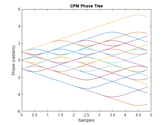
Plot the phase tree diagram for signals that have applied continuous phase modulation (CPM). A phase tree diagram superimposes many curves, each of which plots the phase of a modulated signal over time. The distinct curves result from different inputs to the modulator. This example defines settings for the CPM modulator, applies symbol mapping, and plots the results. Each curve represents a different instance of simulating the CPM modulator with a distinct (constant) input signal.
Define parameters for the example and create a CPM modulator System object™.
M = 2;                   % Modulation order
modindex = 2/3;          % Modulation index
sps = 8;                 % Samples per symbol
L = 5;                   % Symbols to display
pmat = zeros(L*sps,M^L); % Empty phase matrix

cpm = comm.CPMModulator(M, ...
    ModulationIndex=modindex, ...
    FrequencyPulse="Raised Cosine", ...
    PulseLength=2, ...
    SamplesPerSymbol=sps);
Use a for-loop to apply the mapping of the input symbol to the CPM symbols, mapping 0 to -(M-1), 1 to -(M-2), and so on. Populate the columns of the phase matrix with the unwrapped phase angle of the modulated symbols.
for ip_sig = 0:(M^L)-1
    s = int2bit(ip_sig,L,1);
    s = 2*s + 1 - M;
    x = cpm(s);
    pmat(:,ip_sig+1) = unwrap(angle(x(:)));
end
pmat = pmat/(pi*modindex);
t = (0:L*sps-1)'/sps;
Plot the CPM phase tree.
plot(t,pmat);
title('CPM Phase Tree')
xlabel('Samples')
ylabel('Phase (radians)')
View CPM Phase Tree Using Simulink
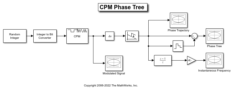
The doc_cpm_phase_tree model uses the Eye Diagram block to view the in-phase and quadrature components, phase trajectory, phase tree, and instantaneous frequency of a CPM modulated signal.
Explore Model
A random integer signal is converted to bits and then CPM modulated. The CPM modulated signal values are converted from complex to magnitude, and angle, and then the phase is unwrapped.
Plot Eye Diagrams
Eye Diagram blocks are named to reflect the signal each displays. When you run the example, these Eye Diagram blocks show how the CPM signal changes over time:
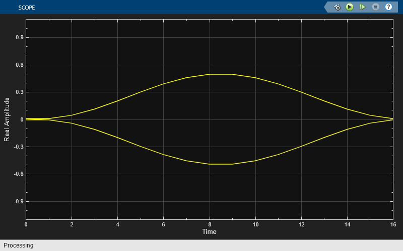
Modulated Signal block — Displays the in-phase and quadrature signals. Double-click the block to open the scope. The modulated signal is easy to see in the eye diagram only when the Modulation index parameter in the CPM Modulator Baseband block is set to 1/2. For a modulation index value of 2/3, the modulation is more complex and the features of the modulated signal are difficult to decipher. Unwrapping the phase and plotting it is another way to illustrate these more complex CPM modulated signals.
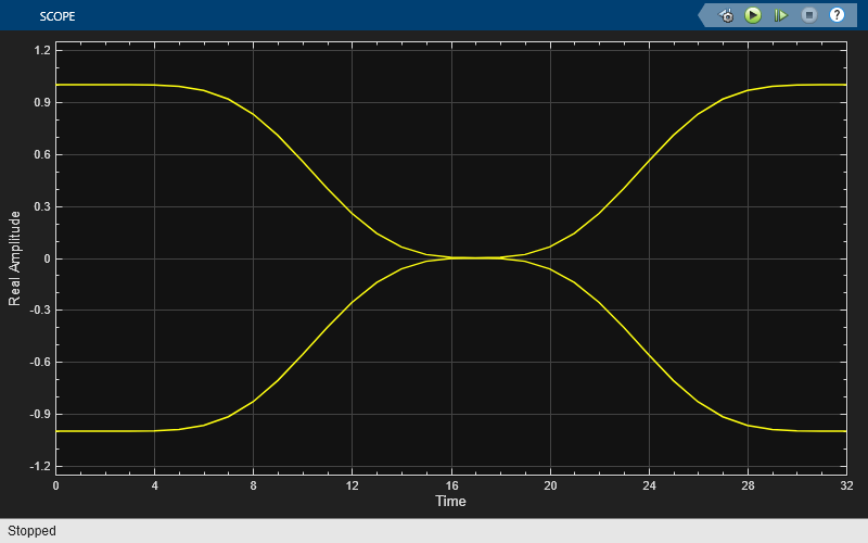
Phase Trajectory block — Displays the CPM phase. Double-click the block to open the scope. The Phase Trajectory block reveals that the signal phase is also difficult to view because it drifts with the data input to the modulator.
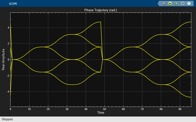
Phase Tree block — Displays the phase tree of the signal. The CPM phase is processed by a few simple blocks to make the CPM pulse shaping easier to view. This processing holds the phase at the beginning of the symbol interval and subtracts it from the signal. This zero-order hold resets the phase to zero every three symbols. The resulting plot shows the many phase trajectories that can be taken by the signal from any given symbol epoch.
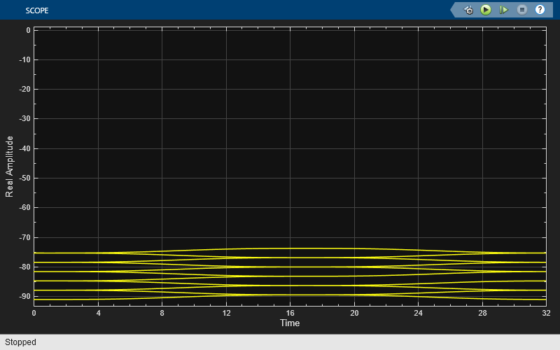
Instantaneous Frequency block — Displays the instantaneous frequency of the signal. The CPM phase is differentiated to produce the frequency deviation of the signal. Viewing the CPM frequency signal enables you to observe the frequency deviation qualitatively, as well as make quantitative observations, such as measuring peak frequency deviation.
Running the doc_cpm_phase_tree model opens and plots the phase tree and instantaneous frequency eye diagram plots.
Further Exploration
To learn more about the example, try changing the following parameters in the CPM Modulator Baseband block:
Change Pulse length to a value between 1 and 6.
Change Frequency pulse shape to one of the other settings, such as
RectangularorGaussian.
You can observe the effect of changing these parameters on the phase tree and instantaneous frequency of the modulated signal.
Compare Filtered QPSK and MSK Signals in Simulink
The cm_qpsk_vs_msk model compares filtered quadrature phase shift keying (QPSK) and minimum shift keying (MSK) modulation schemes.

The model generates the filtered QPSK signal using random integer data from the Random Integer Generator block, which gets modulated by the QPSK Modulator Baseband block, and then filtered by the Raised Cosine Transmit Filter block. The model generates the MSK signal using random binary data from the Bernoulli Binary Generator block, which gets modulated by the MSK Modulator Baseband block. The model adds noise to both the filtered QPSK and MSK signals by using AWGN Channel blocks. The Eye Diagram blocks are used to visualize eye diagrams of both signals.
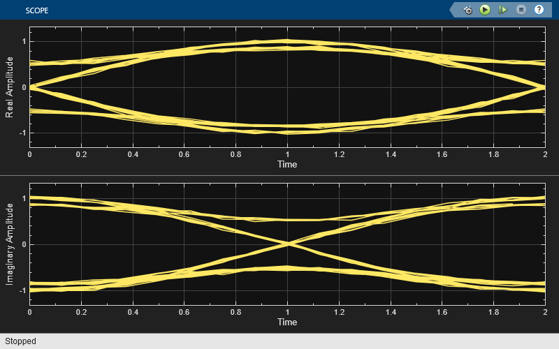
For filtered QPSK modulation, the values of both the in-phase and quadrature components of the signal are permitted to change at any symbol interval. For MSK modulation, the symbol interval is half that for QPSK, but the in-phase and quadrature components change values in alternate symbol epochs.
Compare eye diagram plots of a QPSK-modulated signal and an MSK-modulated signal. For QPSK, the ideal sampling period is 1/2 sample, with sampling time for both in-phase and quadrature signal components at 0.5, 1.5, 2.5, .... For MSK, the ideal sample period is 1 sample, with sampling time at 0.5, 1.5, 2.5, ... for the in-phase signal component and 1, 2, 3, ... for the quadrature signal component.


Compare GMSK and MSK Signals in Simulink
The cm_gmsk_vs_msk model compares Gaussian minimum shift keying (GMSK) and minimum shift keying (MSK) modulation schemes.
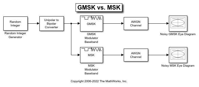
The Random Integer Generator block provides a source of uniformly distributed random integers in the range [0, M-1], where M is the constellation size of the GMSK or MSK signal. The Unipolar to Bipolar Converter block maps a unipolar input signal to a bipolar output signal consisting of integers between -(M-1) and +(M-1). The bipolar data is routed to separate paths. The top path applies GMSK modulation by using the GMSK Modulator Baseband block. The bottom path applies MSK modulation by using the MSK Modulator Baseband block. Noise is added to both the GMSK and MSK signals by using AWGN Channel blocks. The Eye Diagram blocks are used to visualize eye diagrams of both signals.
The eye diagrams show the similarity between the GMSK and MSK signals when you set the initial pulse length of the GMSK Modulator Baseband block to 1.
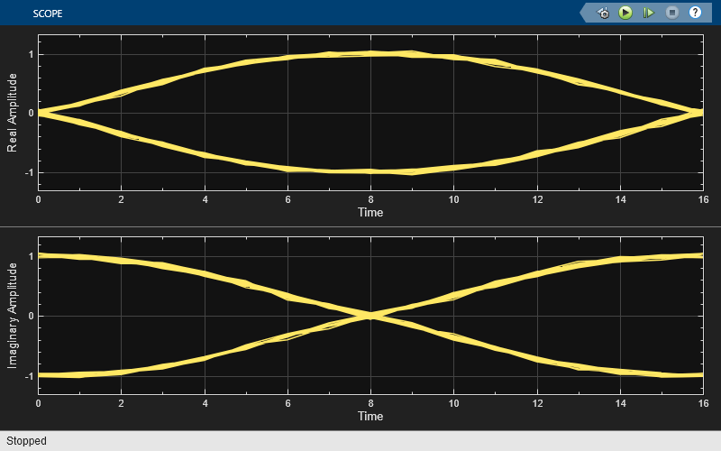
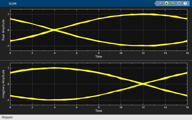
To view the difference that a partial response modulation has on the eye diagram, set the initial pulse length in the GMSK modulator to 5. The increased pulse length results in an increase in the number of paths, showing that the CPM waveform depends on values of the previous symbols as well as the present symbol. Plot the eye diagram of the GMSK signal.
If you change the initial pulse length to an even number, such as 4, you should set the initial phase offset of the GMSK modulator to pi/4 and the offset argument of the eye diagram to 0 for a better view of the modulated signal. To more clearly view the Gaussian pulse shape, you must use scopes that enable you to view the phase of the signal, as described in the View CPM Phase Tree Using Simulink example.

Soft Decision GMSK Demodulator
This model shows a system that includes convolutional coding and GMSK modulation. The receiver in this model includes two parallel paths, one that uses soft decisions and another that uses hard decisions. The model computes bit error rates for the two paths to illustrate that the soft decision receiver performs better. The performance advantage for soft decision reception over hard decision reception is expected because soft decisions enable the system to retain more information from the demodulation operation to use in the decoding operation.
Explore Model
The GMSKSoftDecision model transmits and receives a coded GMSK signal. The key components include the:
Bernoulli Binary Generator block to generate binary numbers for the input signal.
Convolutional Encoder block to encode the binary numbers using a rate 1/2 convolutional code.
Matrix Interleaver block to perform interleaving on coded bits.
GMSK Modulator Baseband block to perform GMSK modulation on interleaved bits.
Pair of
comm.GMSKDemodulatorsystem objects as blocks to perform both hard and soft decision demodulation.Pair of Matrix Deinterleaver blocks for de-interleaving the demodulated output.
Pair of Viterbi Decoder blocks for decoding hard and soft demodulated output.
Pair of Error Rate Calculation blocks, and Display (Simulink) blocks to show the BER for the system with each type of decision.
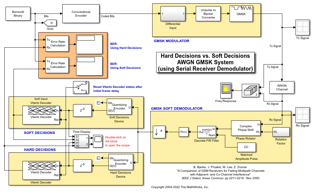
GMSK Receiver
The GMSK demodulator is based on Viterbi-based demodulator. Soft demodulation uses max log MAP BCJR algorithm to calculate log-likelihood ratios. The GMSK waveform used in this model has a BT product of 0.3 and a frequency pulse length of 4 symbols.
Results and Visualizations
To evaluate the performance of soft and hard decision decoding, this example has the following visualizations:
The Display blocks show the BER results to highlight that soft decision receiver performs better than the hard decision receiver.
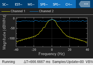
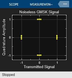
The Tx Signal window shows the scatter plot of the noiseless GMSK signal before the AWGN channel.
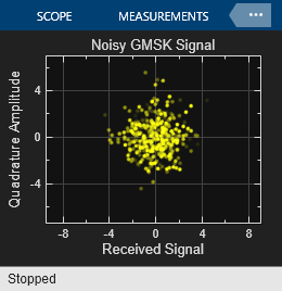
The Rx Signal window shows the scatter plot of the noisy GMSK signal after the AWGN channel.
References
Anderson, John B., Tor Aulin, and Carl-Erik Sundberg. Digital Phase Modulation. New York: Plenum Press, 1986. Benedetto, S., G. Montorsi, D. Divsalar, and F. Pollara.
A Soft-Input Soft-Output Maximum A Posterior (MAP) Module to Decode Parallel and Serial Concatenated Codes, Jet Propulsion Lab TDA Progress Report, November 1996.
Viterbi, A.J. An Intuitive Justification and a Simplified Implementation of the MAP Decoder for Convolutional Codes, IEEE Journal on Selected Areas in Communications 16, no. 2 February 1998.
See Also
Functions
Objects
comm.CPFSKModulator|comm.CPFSKDemodulator|comm.CPMModulator|comm.CPMDemodulator|comm.GMSKModulator|comm.GMSKDemodulator|comm.MSKModulator|comm.MSKDemodulator
Blocks
- CPFSK Modulator Baseband | CPFSK Demodulator Baseband | CPM Modulator Baseband | CPM Demodulator Baseband | GMSK Modulator Baseband | GMSK Demodulator Baseband | MSK Modulator Baseband | MSK Demodulator Baseband