Design an LQG Servo Controller
This example shows you how to design a servo controller for the following system.
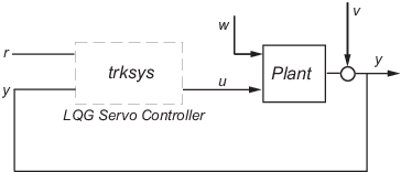
The plant has three states (x), two control inputs (u), two random inputs (w), one output (y), measurement noise for the output (v), and the following state and measurement equations:
where
The system has the following noise covariance data:
Use the following cost function to define the tradeoff between tracker performance and control effort:
To design an LQG servo controller for this system:
Create the state space system by typing the following in the MATLAB® Command Window:
A = [0 1 0;0 0 1;1 0 0];
B = [0.3 1;0 1;-0.3 0.9];
G = [-0.7 1.12; -1.17 1; .14 1.5];
C = [1.9 1.3 1];
D = [0.53 -0.61];
H = [-1.2 -0.89];
sys = ss(A,[B G],C,[D H]);
Construct the optimal state-feedback gain using the given cost function by typing the following commands:
nx = 3;    %Number of states
ny = 1;    %Number of outputs
Q = blkdiag(0.1*eye(nx),eye(ny));
R = [1 0;0 2];
K = lqi(ss(A,B,C,D),Q,R);
Construct the Kalman state estimator using the given noise covariance data by typing the following commands:
Qn = [4 2;2 1];
Rn = 0.7;
kest = kalman(sys,Qn,Rn);
Connect the Kalman state estimator and the optimal state-feedback gain to form the LQG servo controller by typing the following command:
This command returns the following LQG servo controller:trksys = lqgtrack(kest,K)
>> trksys = lqgtrack(kest,K)

a =
           x1_e    x2_e    x3_e     xi1
   x1_e  -2.373  -1.062  -1.649   0.772
   x2_e  -3.443  -2.876  -1.335  0.6351
   x3_e  -1.963  -2.483  -2.043  0.4049
   xi1        0       0       0       0

b =
             r1      y1
   x1_e       0  0.2849
   x2_e       0  0.7727
   x3_e       0  0.7058
   xi1        1      -1

c =
          x1_e     x2_e     x3_e      xi1
   u1  -0.5388  -0.4173  -0.2481   0.5578
   u2   -1.492   -1.388   -1.131   0.5869

d =
       r1  y1
   u1   0   0
   u2   0   0

Input groups:
       Name        Channels
     Setpoint         1
    Measurement       2

Output groups:
      Name      Channels
    Controls      1,2

Continuous-time model.