lqgreg
Form linear-quadratic-Gaussian (LQG) regulator
Syntax
rlqg = lqgreg(kest,k)

rlqg = lqgreg(kest,k,controls)
Description
rlqg = lqgreg(kest,k) returns the LQG regulator
rlqg (a state-space model) given the Kalman estimator
kest and the state-feedback gain matrix k. The same
function handles both continuous- and discrete-time cases. Use consistent tools to design
kest and k:
Continuous regulator for continuous plant: use
lqrorlqryandkalmanDiscrete regulator for discrete plant: use
dlqrorlqryandkalmanDiscrete regulator for continuous plant: use
lqrdandkalmd
In discrete time, lqgreg produces the regulator
when
kestis the "current" Kalman estimatorwhen
kestis the "delayed" Kalman estimator
For more information on Kalman estimators, see the kalman reference page.
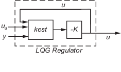
rlqg = lqgreg(kest,k,controls) handles estimators that have access to
additional deterministic known plant inputs ud. The
index vector controls then specifies which estimator inputs are the
controls u, and the resulting LQG regulator rlqg has
ud and y as inputs (see the
next figure).
Note
Always use positive feedback to connect the LQG regulator to the plant.
Examples
See the example LQG Regulation: Rolling Mill Case Study.
Algorithms
lqgreg forms the linear-quadratic-Gaussian (LQG)
regulator by connecting the Kalman estimator designed with kalman and the
optimal state-feedback gain designed with lqr, dlqr, or
lqry. The LQG regulator minimizes some quadratic cost function that
trades off regulation performance and control effort. This regulator is dynamic and relies on
noisy output measurements to generate the regulating commands.
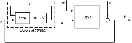
In continuous time, the LQG regulator generates the commands
where is the Kalman state estimate. The regulator state-space equations are
where y is the vector of plant output measurements (see
kalman for background and notation). The following diagram shows this
dynamic regulator in relation to the plant.
In discrete time, you can form the LQG regulator using either the delayed state estimate of x[n], based on measurements up to y[n–1], or the current state estimate , based on all available measurements including y[n]. While the regulator
is always well-defined, the current regulator
is causal only when I-KMD is invertible (see
kalman for the notation). In addition, practical implementations of the
current regulator should allow for the processing time required to compute
u[n] after the measurements
y[n] become available (this amounts to a time delay in
the feedback loop).
For a discrete-time plant with equations:
connecting the "current" Kalman estimator to the LQR gain is optimal only when and y[n] does not depend on
w[n] (H = 0). If these conditions are not satisfied, compute the optimal LQG controller
using lqg.
Version History
Introduced before R2006a