Aerial Lidar Semantic Segmentation Using PointNet++ Deep Learning
This example shows how to train a PointNet++ deep learning network to perform semantic segmentation on aerial lidar data.
Lidar data acquired from airborne laser scanning systems is used in applications such as topographic mapping, city modeling, biomass measurement, and disaster management. Extracting meaningful information from this data requires semantic segmentation, a process where each point in the point cloud is assigned a unique class label.
In this example, you train a PointNet++ network to perform semantic segmentation by using the Dayton Annotated Lidar Earth Scan (DALES) dataset [1]. The dataset contains scenes of dense, labeled aerial lidar data from urban, suburban, rural, and commercial settings. The dataset provides semantic segmentation labels for 8 classes such as buildings, cars, trucks, poles, power lines, fences, ground, and vegetation.
Load DALES Data
The DALES dataset contains 40 scenes of aerial lidar data. Out of the 40 scenes, 29 scenes are used for training and the remaining 11 scenes are used for testing. Each pixel in the data has a class label. Follow the instructions on the DALES website to download the dataset to the folder specified by the dataFolder variable. Create folders to store training and test data.
dataFolder = fullfile(tempdir,'DALES');
trainDataFolder = fullfile(dataFolder,'dales_las','train');
testDataFolder = fullfile(dataFolder,'dales_las','test');
Preview a point cloud from the training data.
lasReader = lasFileReader(fullfile(trainDataFolder,'5080_54435.las'));
[pc,attr] = readPointCloud(lasReader,'Attributes','Classification');
labels = attr.Classification;

% Select only labeled data.
pc = select(pc,labels~=0);
labels = labels(labels~=0);
classNames = [
    "ground"
    "vegetation"
    "cars"
    "trucks"
    "powerlines"
    "fences"
    "poles"
    "buildings"
    ];
figure;
ax = pcshow(pc.Location,labels);
helperLabelColorbar(ax,classNames);
title("Point Cloud with Overlaid Semantic Labels");

Preprocess Data
Each point cloud in the DALES dataset covers an area of 500-by-500 meters, which is much larger than the typical area covered by terrestrial lidar point clouds. For efficient memory processing, divide the point cloud into small, non-overlapping blocks by using a blockedPointCloud (Lidar Toolbox) object.
Define the block dimensions using the blockSize parameter. As the size of each point cloud in the dataset varies, set the z-dimension of the block to Inf to avoid block creation along z-axis.
blocksize = [51 51 Inf];
Create a matlab.io.datastore.FileSet object to collect all the point cloud files in the training data.
fs = matlab.io.datastore.FileSet(trainDataFolder);
Create a blockedPointCloud (Lidar Toolbox) object using the Fileset object.
bpc = blockedPointCloud(fs,blocksize);
Note: Processing can take some time. The code suspends MATLAB® execution until processing is complete.
Use the helperCalculateClassWeights helper function, attached to this example as a supporting file, to calculate the point distribution across all the classes in the training dataset.
numClasses = numel(classNames);
[weights,maxLabel,maxWeight] = helperCalculateClassWeights(fs,numClasses);
Create Datastore Object for Training
Create a blockedPointCloudDatastore (Lidar Toolbox) object using the blocked point cloud, bpc to train the network.
ldsTrain = blockedPointCloudDatastore(bpc,MinPoints=10);
Specify label IDs from 1 to the number of classes.
labelIDs = 1 : numClasses;
Preview and display the point cloud.
ptcld = preview(ldsTrain);
figure;
pcshow(ptcld.Location);
title("Cropped Point Cloud");
For faster training, set a fixed number of points per block.
numPoints = 8192;
Transform the data to make it compatible with the input layer of the network, using the helperTransformToTrainData function, defined at the end of this example. Follow these steps to apply transformation.
Extract the point cloud and the respective labels.
Downsample the point cloud, the labels to a specified number,
numPoints.Normalize the point clouds to the range [0 1].
Convert the point cloud and the corresponding labels to make them compatible with the input layer of the network.
ldsTransformed = transform(ldsTrain,@(x,info) helperTransformToTrainData(x, ...
    numPoints,info,labelIDs,classNames),'IncludeInfo',true);
read(ldsTransformed)
ans=1×2 cell array
    8192×3 double    8192×1 categorical
Define PointNet++ Model
PointNet++ is a popular neural network used for semantic segmentation of unorganized lidar point clouds. Semantic segmentation associates each point in a 3-D point cloud with a class label, such as car, truck, ground, or vegetation. For more information, see Get Started with PointNet++ (Lidar Toolbox).
Define the PointNet++ architecture using the pointnetplusNetwork function.
net = pointnetplusNetwork(numPoints,3,numClasses);
To handle the class-imbalance on the DALES dataset, the weighted crossentropy loss function is used. This will penalize the network more if a point that belongs to a class with lower weight is misclassified.
% Define the loss function.
lossfun = @(Y,T) mean(mean(sum(crossentropy(Y,T,weights,'WeightsFormat','UC','Reduction','none'),3),1),4);
Specify Training Options
Use the Adam optimization algorithm to train the network. Use the trainingOptions function to specify the hyperparameters.
Train the network using a CPU or GPU. Using a GPU requires Parallel Computing Toolbox™ and a CUDA® enabled NVIDIA® GPU. For more information, see GPU Computing Requirements (Parallel Computing Toolbox). To automatically detect if you have a GPU available, set executionEnvironment to "auto". If you do not have a GPU, or do not want to use one for training, set executionEnvironment to "cpu". To ensure the use of a GPU for training, set executionEnvironment to "gpu".
executionEnvironment = "auto";
if canUseParallelPool
    dispatchInBackground = true;
else
    dispatchInBackground = false;
end

learningRate = 0.0005;
l2Regularization = 0.01;
numEpochs = 20;
miniBatchSize = 16;
learnRateDropFactor = 0.1;
learnRateDropPeriod = 10;
gradientDecayFactor = 0.9;
squaredGradientDecayFactor = 0.999;

options = trainingOptions('adam', ...
    'InitialLearnRate',learningRate, ...
    'L2Regularization',l2Regularization, ...
    'MaxEpochs',numEpochs, ...
    'MiniBatchSize',miniBatchSize, ...
    'LearnRateSchedule','piecewise', ...
    'LearnRateDropFactor',learnRateDropFactor, ...
    'LearnRateDropPeriod',learnRateDropPeriod, ...
    'GradientDecayFactor',gradientDecayFactor, ...
    'SquaredGradientDecayFactor',squaredGradientDecayFactor, ...
    'ExecutionEnvironment',executionEnvironment, ...
    'DispatchInBackground',dispatchInBackground, ...
    'Plots','training-progress');
Note: Reduce the miniBatchSize value to control memory usage when training.
Train Model
To train the network, set the doTraining argument to true. Otherwise, load a pretrained network. To train the network, you can use CPU or GPU. Using a GPU requires Parallel Computing Toolbox™ and a CUDA® enabled NVIDIA® GPU. For more information, see GPU Computing Requirements (Parallel Computing Toolbox).
doTraining = false;
if doTraining
    % Train the network on the ldsTransformed datastore using
    % the trainnet function.
    [net,info] = trainnet(ldsTransformed,net,lossfun,options);
else
    % Load the pretrained network.
    load('pointnetplusNetworkTrained','net');
end
Segment Aerial Point Cloud
To perform segmentation on the test point cloud, first create a blockedPointCloud (Lidar Toolbox) object, then create a blockedPointCloudDatastore (Lidar Toolbox) object.
Apply the similar transformation used on training data, to the test data:
Extract the point cloud and the respective labels.
Downsample the point cloud to a specified number,
numPoints.Normalize the point clouds to the range [0 1].
Convert the point cloud to make it compatible with the input layer of the network.
tbpc = blockedPointCloud(fullfile(testDataFolder,'5080_54470.las'),blocksize);
tbpcds = blockedPointCloudDatastore(tbpc);
Define numNearestNeighbors and radius to find the nearest points in the downsampled point cloud for each point in the dense point cloud and to perform interpolation effectively.
numNearestNeighbors = 20;
radius = 0.05;
Initialize empty placeholder for predictions.
labelsDensePred = [];
Perform inference on this test point cloud to compute prediction labels. Interpolate the prediction labels, to obtain prediction labels on the dense point cloud. Iterate the process all over the non-overlapping blocks and predict the labels using the pcsemanticseg (Lidar Toolbox) function.
while hasdata(tbpcds)

    % Read the block along with block information.
    ptCloudDense = read(tbpcds);

    % Use the helperDownsamplePoints function, attached to this example as a
    % supporting file, to extract a downsampled point cloud from the
    % dense point cloud.
    ptCloudSparse = helperDownsamplePoints(ptCloudDense{1},[],numPoints);

    % Use the helperNormalizePointCloud function, attached to this example as
    % a supporting file, to normalize the point cloud between 0 and 1.
    ptCloudSparseNormalized = helperNormalizePointCloud(ptCloudSparse);
    ptCloudDenseNormalized = helperNormalizePointCloud(ptCloudDense{1});

    % Use the helperTransformToTestData function, defined at the end of this
    % example, to convert the point cloud to a cell array and to permute the
    % dimensions of the point cloud to make it compatible with the input layer
    % of the network.
    ptCloudSparseForPrediction = helperTransformToTestData(ptCloudSparseNormalized);

    % Get the output predictions.
    labelsSparsePred = predict(net,ptCloudSparseForPrediction{1,1});
    [~,labelsSparsePred] = max(labelsSparsePred,[],3);

    % Use the helperInterpolate function, attached to this example as a
    % supporting file, to calculate labels for the dense point cloud,
    % using the sparse point cloud and labels predicted on the sparse point cloud.
    interpolatedLabels = helperInterpolate(ptCloudDenseNormalized, ...
        ptCloudSparseNormalized,labelsSparsePred,numNearestNeighbors, ...
        radius,maxLabel,numClasses);

    % Concatenate the predicted labels from the blocks.
    labelsDensePred = vertcat(labelsDensePred,interpolatedLabels);
end
Starting parallel pool (parpool) using the 'Processes' profile ...
Connected to parallel pool with 32 workers.
For better visualization, only display a block inferred from the point cloud data.
figure;
ax = pcshow(ptCloudDense{1}.Location,interpolatedLabels);
axis off;
helperLabelColorbar(ax,classNames);
title("Point Cloud Overlaid with Detected Semantic Labels");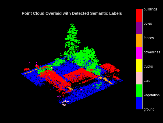
Evaluate Network
To perform evaluation on the test data, get the labels from the test point cloud. The labels for the test data are already predicted in the previous step. Hence, iterate over the non-overlapping blocks of the point cloud and extract the ground truth labels.
Initialize the placeholders for target labels.
labelsDenseTarget = [];
Loop over the block point cloud datastore and get the ground truth labels.
reset(tbpcds);

while hasdata(tbpcds)
    % Read the block along with block information.
    [~,infoDense] = read(tbpcds);

    % Extract the labels from the block information.
    labelsDense = infoDense.PointAttributes.Classification;

    % Concatenate the target labels from the blocks.
    labelsDenseTarget = vertcat(labelsDenseTarget,labelsDense);
end
Use the evaluateSemanticSegmentation (Computer Vision Toolbox) function to compute the semantic segmentation metrics from the test set results. The target and predicted labels are computed previously and are stored in the labelsDensePred and the labelsDenseTarget variables respectively.
confusionMatrix = segmentationConfusionMatrix(double(labelsDensePred), ...
    double(labelsDenseTarget),'Classes',1:numClasses);
metrics = evaluateSemanticSegmentation({confusionMatrix},classNames,'Verbose',false);
You can measure the amount of overlap per class using the intersection-over-union (IoU) metric.
The evaluateSemanticSegmentation (Computer Vision Toolbox) function returns metrics for the entire data set, for individual classes, and for each test image. To see the metrics at the data set level, use the metrics.DataSetMetrics property.
metrics.DataSetMetrics
ans=1×4 table
    0.9365    0.6649    0.5344    0.8905
The data set metrics provide a high-level overview of network performance. To see the impact each class has on the overall performance, inspect the metrics for each class using the metrics.ClassMetrics property.
metrics.ClassMetrics
ans=8×2 table
    0.9925    0.9430
    0.8580    0.8318
    0.5780    0.4079
    0.1588    0.0564
    0.7577    0.6736
    0.5040    0.2406
    0.5305    0.2238
    0.9399    0.8980
Although the overall network performance is good, the class metrics for some classes like Trucks indicate that more training data is required for better performance.
Supporting Functions
The helperLabelColorbar function adds a colorbar to the current axis. The colorbar is formatted to display the class names with the color.
function helperLabelColorbar(ax,classNames)
% Colormap for the original classes.
cmap = [[0 0 255];
    [0 255 0];
    [255 192 203];
    [255 255 0];
    [255 0 255];
    [255 165 0];
    [139 0 150];
    [255 0 0]];
cmap = cmap./255;
cmap = cmap(1:numel(classNames),:);
colormap(ax,cmap);

% Add colorbar to current figure.
c = colorbar(ax);
c.Color = 'w';

% Center tick labels and use class names for tick marks.
numClasses = size(classNames,1);
c.Ticks = 1:1:numClasses;
c.TickLabels = classNames;

% Remove tick mark.
c.TickLength = 0;
end
The helperTransformToTrainData function performs these set of transforms on the input data which are:
Extract the point cloud and the respective labels.
Downsample the point cloud, the labels to a specified number,
numPoints.Normalize the point clouds to the range [0 1].
Convert the point cloud and the corresponding labels to make them compatible with the input layer of the network.
function [cellout,dataout] = helperTransformToTrainData(data,numPoints,info,...
    labelIDs,classNames)
if ~iscell(data)
    data = {data};
end
numObservations = size(data,1);
cellout = cell(numObservations,2);
dataout = cell(numObservations,2);
for i = 1:numObservations
    classification = info.PointAttributes(i).Classification;

    % Remove labels with zero value.
    pc = data{i,1};
    pc = select(pc,(classification ~= 0));
    classification = classification(classification ~= 0);

    % Use the helperDownsamplePoints function, attached to this example as a
    % supporting file, to extract a downsampled point cloud and its labels
    % from the dense point cloud.
    [ptCloudOut,labelsOut] = helperDownsamplePoints(pc, ...
    classification,numPoints);

    % Make the spatial extent of the dense point cloud and the sparse point
    % cloud same.
    limits = [ptCloudOut.XLimits;ptCloudOut.YLimits;...
                    ptCloudOut.ZLimits];
    ptCloudSparseLocation = ptCloudOut.Location;
    ptCloudSparseLocation(1:2,:) = limits(:,1:2)';
    ptCloudSparseUpdated = pointCloud(ptCloudSparseLocation, ...
        'Intensity',ptCloudOut.Intensity, ...
        'Color',ptCloudOut.Color, ...
        'Normal',ptCloudOut.Normal);

    % Use the helperNormalizePointCloud function, attached to this example as
    % a supporting file, to normalize the point cloud between 0 and 1.
    ptCloudOutSparse = helperNormalizePointCloud( ...
        ptCloudSparseUpdated);
    cellout{i,1} = ptCloudOutSparse.Location;

    % Permuted output.
    cellout{i,2} = permute(categorical(labelsOut,labelIDs,classNames),[1 3 2]);

    % General output.
    dataout{i,1} = ptCloudOutSparse;
    dataout{i,2} = labelsOut;
end
end
The helperTransformToTestData function converts the point cloud to a cell array and permutes the dimensions of the point cloud to make it compatible with the input layer of the network.
function data = helperTransformToTestData(data)
if ~iscell(data)
    data = {data};
end
numObservations = size(data,1);
for i = 1:numObservations
    tmp = data{i,1}.Location;
    data{i,1} = tmp;
end
end
References
[1] Varney, Nina, Vijayan K. Asari, and Quinn Graehling. "DALES: A Large-Scale Aerial LiDAR dataset for Semantic Segmentation." ArXiv:2004.11985 [Cs, Stat], April 14, 2020. https://arxiv.org/abs/2004.11985.
[2] Qi, Charles R., Li Yi, Hao Su, and Leonidas J. Guibas. "PointNet++: Deep Hierarchical Feature Learning on Point Sets in a Metric Space." ArXiv:1706.02413 [Cs], June 7, 2017. https://arxiv.org/abs/1706.02413.