Simulate States of Time-Varying State-Space Model Using Simulation Smoother
This example generates data from a known model, fits a state-space model to the data, and then simulates series from the fitted model using the simulation smoother.
Suppose that a latent process comprises an AR(2) and an MA(1) model. There are 50 periods, and the MA(1) process drops out of the model for the final 25 periods. The state equation for the first 25 periods is
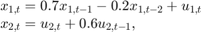
and for the last 25 periods, it is

where  and
and  are Gaussian with mean 0 and standard deviation 1.
Assuming that the series starts at 1.5 and 1, respectively, generate a random series of 50 observations from  and
and  .
.
T = 50;
ARMdl = arima('AR',{0.7,-0.2},'Constant',0,'Variance',1);
MAMdl = arima('MA',0.6,'Constant',0,'Variance',1);
x0 = [1.5 1; 1.5 1];
rng(1);
x = [simulate(ARMdl,T,'Y0',x0(:,1)),...
    [simulate(MAMdl,T/2,'Y0',x0(:,2));nan(T/2,1)]];
The last 25 values for the simulated MA(1) data are NaN values.
Suppose further that the latent processes are measured using
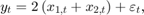
for the first 25 periods, and

for the last 25 periods, where  is Gaussian with mean 0 and standard deviation 1.
Use the random latent state process (x) and the observation equation to generate observations.
y = 2*sum(x','omitnan')'+randn(T,1);
Together, the latent process and observation equations compose a state-space model. Supposing that the coefficients are unknown parameters, the state-space model is
![$$\begin{array}{l} \left[ {\begin{array}{*{20}{c}} {{x_{1,t}}}\\ {{x_{2,t}}}\\ {{x_{3,t}}}\\ {{x_{4,t}}} \end{array}} \right] = \left[ {\begin{array}{*{20}{c}} {{\phi _1}}&{{\phi _2}}&0&0\\ 1&0&0&0\\ 0&0&0&{{\theta _1}}\\ 0&0&0&0 \end{array}} \right]\left[ {\begin{array}{*{20}{c}} {{x_{1,t - 1}}}\\ {{x_{2,t - 1}}}\\ {{x_{3,t - 1}}}\\ {{x_{4,t - 1}}} \end{array}} \right] + \left[ {\begin{array}{*{20}{c}} 1&0\\ 0&0\\ 0&1\\ 0&1 \end{array}} \right]\left[ {\begin{array}{*{20}{c}} {{u_{1,t}}}\\ {{u_{2,t}}} \end{array}} \right]\\ {y_t} = a({x_{1,t}} + {x_{3,t}}) + {\varepsilon _t} \end{array}$$](../examples/econ/win64/SimulateStatesOfTimeVaryingStateSpaceExample_eq08939596656225341196.png)
for the first 25 periods,
![$$\begin{array}{l} \left[ {\begin{array}{*{20}{c}} {{x_{1,t}}}\\ {{x_{2,t}}} \end{array}} \right] = \left[ {\begin{array}{*{20}{c}} {{\phi _1}}&{{\phi _2}}&0&0\\ 1&0&0&0 \end{array}} \right]\left[ {\begin{array}{*{20}{c}} {{x_{1,t - 1}}}\\ {{x_{2,t - 1}}}\\ {{x_{3,t - 1}}}\\ {{x_{4,t - 1}}} \end{array}} \right] + \left[ {\begin{array}{*{20}{c}} 1\\ 0 \end{array}} \right]{u_{1,t}}\\ {y_t} = b{x_{1,t}} + {\varepsilon _t} \end{array}$$](../examples/econ/win64/SimulateStatesOfTimeVaryingStateSpaceExample_eq14434019549381870163.png)
for period 26, and
![$$\begin{array}{l} \left[ {\begin{array}{*{20}{c}} {{x_{1,t}}}\\ {{x_{2,t}}} \end{array}} \right] = \left[ {\begin{array}{*{20}{c}} {{\phi _1}}&{{\phi _2}}\\ 1&0 \end{array}} \right]\left[ {\begin{array}{*{20}{c}} {{x_{1,t - 1}}}\\ {{x_{2,t - 1}}} \end{array}} \right] + \left[ {\begin{array}{*{20}{c}} 1\\ 0 \end{array}} \right]{u_{1,t}}\\ {y_t} = b{x_{1,t}} + {\varepsilon _t} \end{array}$$](../examples/econ/win64/SimulateStatesOfTimeVaryingStateSpaceExample_eq14967989555778478098.png)
for the last 24 periods.
Write a function that specifies how the parameters in params map to the state-space model matrices, the initial state values, and the type of state.
% Copyright 2015 The MathWorks, Inc.

function [A,B,C,D,Mean0,Cov0,StateType] = AR2MAParamMap(params,T)
%AR2MAParamMap Time-variant state-space model parameter mapping function
%
% This function maps the vector params to the state-space matrices (A, B,
% C, and D), the initial state value and the initial state variance (Mean0
% and Cov0), and the type of state (StateType). From periods 1 to T/2, the
% state model is an AR(2) and an MA(1) model, and the observation model is
% the sum of the two states. From periods T/2 + 1 to T, the state model is
% just the AR(2) model.
    A1 = {[params(1) params(2) 0 0; 1 0 0 0; 0 0 0 params(3); 0 0 0 0]};
    B1 = {[1 0; 0 0; 0 1; 0 1]};
    C1 = {params(4)*[1 0 1 0]};
    Mean0 = ones(4,1);
    Cov0 = 10*eye(4);
    StateType = [0 0 0 0];
    A2 = {[params(1) params(2) 0 0; 1 0 0 0]};
    B2 = {[1; 0]};
    A3 = {[params(1) params(2); 1 0]};
    B3 = {[1; 0]};
    C3 = {params(5)*[1 0]};
    A = [repmat(A1,T/2,1);A2;repmat(A3,(T-2)/2,1)];
    B = [repmat(B1,T/2,1);B2;repmat(B3,(T-2)/2,1)];
    C = [repmat(C1,T/2,1);repmat(C3,T/2,1)];
    D = 1;
end
Save this code as a file named AR2MAParamMap on your MATLAB® path.
Create the state-space model by passing the function AR2MAParamMap as a function handle to ssm.
Mdl = ssm(@(params)AR2MAParamMap(params,T));
ssm implicitly creates the state-space model. Usually, you cannot verify an implicitly defined state-space model.
Simulate one path of states from Mdl using the simulation smoother. Specify that the parameter-to-matrix mapping function has seven output arguments. Also, specify the unknown values of the parameters.
simParams = [0.48 0.0081 0.56 1.63 1.9];
X = simsmooth(Mdl,y,'NumOut',7,'Params',simParams);
X is a T-by-1 cell vector of simulated states. Cells 1 through 25 contain 4-by-1 vectors, and cells 26 through 50 contain 2-by-1 vectors.
Access a cell using cell indexing, for example, access cell 5 using X{5}.
simStatesPeriod5 = X{5}
simStatesPeriod5 =

   -1.7591
   -1.5404
   -1.5171
   -1.1417
See Also
ssm | simulate | estimate | refine | simsmooth