Managing Interest-Rate Risk with Bond Futures
This example shows how to hedge the interest-rate risk of a portfolio using bond futures.
Modifying the Duration of a Portfolio with Bond Futures
In managing a bond portfolio, you can use a benchmark portfolio to evaluate performance. Sometimes a manager is constrained to keep the portfolio's duration within a particular band of the duration of the benchmark. One way to modify the duration of the portfolio is to buy and sell bonds, however, there may be reasons why a portfolio manager wishes to maintain the existing composition of the portfolio (for example, the current holdings reflect fundamental research/views about future returns). Therefore, another option for modifying the duration is to buy and sell bond futures.
Bond futures are futures contracts where the commodity to be delivered is a government bond that meets the standard outlined in the futures contract (for example, the bond has a specified remaining time to maturity). Since often many bonds are available, and each bond may have a different coupon, you can use a conversion factor to normalize the payment by the long to the short.
There exist well developed markets for government bond futures. Specifically, the Chicago Board of Trade offers futures on the following:
2 Year Note
3 Year Note
5 Year Note
10 Year Note
30 Year Bond
https://www.cmegroup.com/trading/interest-rates/
Eurex offers futures on the following:
Euro-Schatz Futures 1.75 to 2.25
Euro-Bobl Futures 4.5 to 5.5
Euro-Bund Futures 8.5 to 10.5
Euro-Buxl Futures 24.0 to 35
Bond futures can be used to modify the duration of a portfolio. Since bond futures derive their value from the underlying instrument, the duration of a bond futures contract is related to the duration of the underlying bond.
There are two challenges in computing this duration:
Since there are many available bonds for delivery, the short in the contract has a choice in which bond to deliver.
Some contracts allow the short flexibility in choosing the delivery date.
Typically, the bond used for analysis is the bond that is cheapest for the short to deliver (CTD). One approach is to compute duration measures using the CTD's duration and the conversion factor.
For example, the Present Value of a Basis Point (PVBP) can be computed from the following:
Note that these definitions of duration for the futures contract are approximate, and do not account for the value of the delivery options for the short.
If the goal is to modify the duration of a portfolio, use the following:
Note that the contract size is typically for 100,000 face value of a bond -- so the contract size is typically 1000, as the bond face value is 100.
The following example assumes an initial duration, portfolio value, and target duration for a portfolio with exposure to the Euro interest rate. The June Euro-Bund Futures contract is used to modify the duration of the portfolio. Note that typically futures contracts are offered for March, June, September and December.
% Assume the following for the portfolio and target
PortfolioDuration = 6.4;
PortfolioValue = 100000000;
BenchmarkDuration = 4.8;

% Deliverable Bunds -- note that these conversion factors may also be
% computed with the MATLAB(R) function convfactor
BondPrice = [106.46;108.67;104.30];
BondMaturity = datenum({'04-Jan-2018','04-Jul-2018','04-Jan-2019'});
BondCoupon = [.04;.0425;.0375];
ConversionFactor = [.868688;.880218;.839275];

% Futures data -- found from http://www.eurex.com
FuturesPrice = 122.17;
FuturesSettle = '23-Apr-2009';
FuturesDelivery = '10-Jun-2009';

% To find the CTD bond we can compute the implied repo rate
ImpliedRepo = bndfutimprepo(BondPrice,FuturesPrice,FuturesSettle,...
    FuturesDelivery,ConversionFactor,BondCoupon,BondMaturity);

% Note that the bond with the highest implied repo rate is the CTD
[CTDImpRepo,CTDIndex] = max(ImpliedRepo);

% Compute the CTD's Duration -- note the period and basis for German Bunds
Duration = bnddurp(BondPrice,BondCoupon,FuturesSettle,BondMaturity,1,8);

ContractSize = 1000;

% Use the formula above to compute the number of contracts to sell
NumContracts = (BenchmarkDuration - PortfolioDuration)*PortfolioValue./...
    (BondPrice(CTDIndex)*ContractSize*Duration(CTDIndex))*ConversionFactor(CTDIndex);

disp(['To achieve the target duration, ' num2str(abs(round(NumContracts))) ...
    ' Euro-Bund Futures must be sold.'])
To achieve the target duration, 180 Euro-Bund Futures must be sold.
Modifying the Key Rate Durations of a Portfolio with Bond Futures
One of the shortcomings of using duration as a risk measure is that it assumes parallel shifts in the yield curve. While many studies have shown that this explains roughly 85% of the movement in the yield curve, changes in the slope or shape of the yield curve are not captured by duration, and therefore, hedging strategies are not successful at addressing these dynamics. One approach is to use key rate duration -- this is particularly relevant when using bond futures with multiple maturities, like Treasury futures.
The following example uses 2, 5, 10 and 30 year Treasury Bond futures to hedge the key rate duration of a portfolio. Computing key rate durations requires a zero curve. This example uses the zero curve published by the Treasury and found at the following location:
Note that this zero curve could also be derived using the Interest-Rate Curve functionality found in IRDataCurve and IRFunctionCurve.
% Assume the following for the portfolio and target, where the duration
% vectors are key rate durations at 2, 5, 10, and 30 years.
PortfolioDuration = [.5 1 2 6];
PortfolioValue = 100000000;
BenchmarkDuration = [.4 .8 1.6 5];

% The following are the CTD Bonds for the 30, 10, 5 and 2 year futures
% contracts -- these were determined using the procedure outlined in the
% previous section.
CTDCoupon = [4.75 3.125 5.125 7.5]'/100;
CTDMaturity = datenum({'3/31/2011','08/31/2013','05/15/2016','11/15/2024'});
CTDConversion = [0.9794 0.8953 0.9519 1.1484]';
CTDPrice = [107.34 105.91 117.00 144.18]';

ZeroRates = [0.07 0.10 0.31 0.50 0.99 1.38 1.96 2.56 3.03 3.99 3.89]'/100;
ZeroDates = daysadd(FuturesSettle,[30 360 360*2 360*3 360*5 ...
    360*7 360*10 360*15 360*20 360*25 360*30],1);

% Compute the key rate durations for each of the CTD bonds.
CTDKRD = bndkrdur([ZeroDates ZeroRates], CTDCoupon,FuturesSettle,...
    CTDMaturity,'KeyRates',[2 5 10 30]);

% Note that the contract size for the 2 Year Note Future is $200,000
ContractSize = [2000;1000;1000;1000];

NumContracts = (bsxfun(@times,CTDPrice.*ContractSize./CTDConversion,CTDKRD))\...
    (BenchmarkDuration - PortfolioDuration)'*PortfolioValue;

sprintf(['To achieve the target duration, \n' ...
    num2str(-round(NumContracts(1))) ' 2 Year Treasury Note Futures must be sold, \n' ...
    num2str(-round(NumContracts(2))) ' 5 Year Treasury Note Futures must be sold, \n' ...
    num2str(-round(NumContracts(3))) ' 10 Year Treasury Note Futures must be sold, \n' ...
    num2str(-round(NumContracts(4))) ' Treasury Bond Futures must be sold, \n'])
ans =
    'To achieve the target duration,
     24 2 Year Treasury Note Futures must be sold,
     47 5 Year Treasury Note Futures must be sold,
     68 10 Year Treasury Note Futures must be sold,
     120 Treasury Bond Futures must be sold,
     '
Improving the Performance of a Hedge with Regression
An additional component to consider in hedging interest-rate risk with bond futures, again related to movements in the yield curve, is that typically the yield curve moves more at the short end than at the long end.
Therefore, if a position is hedged with a future where the CTD bond has a maturity that is different than the portfolio this could lead to a situation where the hedge under- or over-compensates for the actual interest-rate risk of the portfolio One approach is to perform a regression on historical yields at different maturities to determine a Yield Beta, which is a value that represents how much more the yield changes for different maturities.
This example shows how to use this approach with UK Long Gilt futures and historical data on Gilt Yields.
Market data on Gilt futures is found at the following:
Historical data on gilts is found at the following;
Note that while this approach does offer the possibility of improving the performance of a hedge, any analysis using historical data depends on historical relationships remaining consistent.
Also note that an additional enhancement takes into consideration the correlation between different maturities. While this approach is outside the scope of this example, you can use this to implement a minimum variance hedge.
% Assume the following for the portfolio and target
PortfolioDuration = 6.4;
PortfolioValue = 100000000;
BenchmarkDuration = 4.8;

% This is the CTD Bond for the Long Gilt Futures contract
CTDBondPrice = 113.40;
CTDBondMaturity = datenum('7-Mar-2018');
CTDBondCoupon = .05;
CTDConversionFactor = 0.9325024;

% Market data for the Long Gilt Futures contract
FuturesPrice = 120.80;
FuturesSettle = '23-Apr-2009';
FuturesDelivery = '10-Jun-2009';

CTDDuration = bnddurp(CTDBondPrice,CTDBondCoupon,FuturesSettle,CTDBondMaturity);

ContractSize = 1000;

NumContracts = (BenchmarkDuration - PortfolioDuration)*PortfolioValue./...
    (CTDBondPrice*ContractSize*CTDDuration)*CTDConversionFactor;

disp(['To achieve the target duration with a conventional hedge ' ...
    num2str(-round(NumContracts)) ...
    ' Long Gilt Futures must be sold.'])
To achieve the target duration with a conventional hedge 182 Long Gilt Futures must be sold.
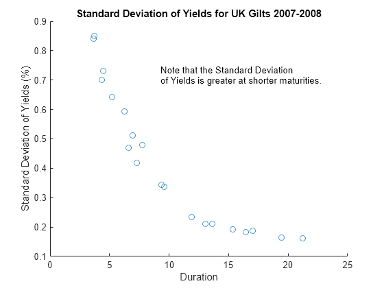
To improve the accuracy of this hedge, historical data is used to determine a relationship between the standard deviation of the yields. Specifically, standard deviation of yields is plotted and regressed vs bond duration. This relationship is then used to compute a Yield Beta for the hedge.
% Load data from XLS spreadsheet
load ukbonddata_20072008

Duration = bnddury(Yield(1,:)',Coupon,Dates(1,:),Maturity);

scatter(Duration,100*std(Yield))
title('Standard Deviation of Yields for UK Gilts 2007-2008')
ylabel('Standard Deviation of Yields (%)')
xlabel('Duration')
annotation(gcf,'textbox',[0.4067 0.685 0.4801 0.0989],...
    'String',{'Note that the Standard Deviation',...
    'of Yields is greater at shorter maturities.'},...
    'FitBoxToText','off',...
    'EdgeColor','none');
stats = regstats(std(Yield),Duration);
YieldBeta = (stats.beta'*[1 PortfolioDuration]')./(stats.beta'*[1 CTDDuration]');
Now the Yield Beta is used to compute a new value for the number of contracts to be sold. Note that since the duration of the portfolio was less than the duration of the CTD Gilt, the number of futures to sell is actually greater than in the first case.
NumContracts = (BenchmarkDuration - PortfolioDuration)*PortfolioValue./...
    (CTDBondPrice*ContractSize*CTDDuration)*CTDConversionFactor*YieldBeta;

disp(['To achieve the target duration using a Yield Beta-modified hedge, ' ...
    num2str(abs(round(NumContracts))) ...
    ' Long Gilt Futures must be sold.'])
To achieve the target duration using a Yield Beta-modified hedge, 193 Long Gilt Futures must be sold.
Bibliography
This example is based on the following books and papers:
[1] Burghardt, G., T. Belton, M. Lane and J. Papa. The Treasury Bond Basis. New York, NY: McGraw-Hill, 2005.
[2] Krgin, D. Handbook of Global Fixed Income Calculations. New York, NY: John Wiley & Sons, 2002.
[3] CFA Program Curriculum, Level III, Volume 4, Reading 31. CFA Institute, 2009.
See Also
capbyblk | floorbyblk | swaptionbyblk | blackvolbysabr | optsensbysabr | agencyoas | agencyprice | bndfutimprepo | bndfutprice | convfactor | tfutbyprice | tfutbyyield | tfutimprepo | tfutpricebyrepo | tfutyieldbyrepo | capbylg2f | floorbylg2f | swaptionbylg2f | blackvolbyrebonato | hwcalbycap | hwcalbyfloor
Topics
- Calibrate the SABR Model
- Price a Swaption Using the SABR Model
- Computing the Agency OAS for Bonds
- Analysis of Bond Futures
- Fitting the Diebold Li Model
- Price Swaptions with Interest-Rate Models Using Simulation
- Managing Present Value with Bond Futures
- Supported Interest-Rate Instrument Functions
- Supported Equity Derivative Functions
- Supported Energy Derivative Functions
- Mapping Financial Instruments Toolbox Functions for Interest-Rate Instrument Objects