Implement FIR Filter Algorithm for Floating-Point and Fixed-Point Types Using cast and zeros
This example shows you how to convert a finite impulse-response (FIR) filter to fixed point by separating the fixed-point type specification from the algorithm code.
Separating data type specification from algorithm code allows you to:
Re-use your algorithm code with different data types
Keep your algorithm uncluttered with data type specification and switch statements for different data types
Keep your algorithm code more readable
Switch between fixed point and floating point to compare baselines
Switch between variations of fixed-point settings without changing the algorithm code
Original FIR Filter Algorithm
This example converts MATLAB® code for a finite impulse response (FIR) filter to fixed point.
The formula for the nth output, y(n), of an FIR filter given filter coefficients b and input x is:
y(n) = b(1)*x(n) + b(2)*x(n-1) + ... + b(end)*x(n-length(b)+1)
Linear Buffer Implementation
There are several different ways to write an FIR filter. One way is with a linear buffer like in the following function, where b is a row vector and z is a column vector the same length as b.
function [y,z] = fir_filt_linear_buff(b,x,z)
    y = zeros(size(x));
    for n=1:length(x)
        z = [x(n); z(1:end-1)];
        y(n) = b * z;
    end
end
The vector z is made up of the current and previous samples of x.
z = [x(n); x(n-1); .. ; x(n-length(b)+1)]
The vector z is called a state vector. It is used as both an input and an output. When it is an input, it is the initial state of the filter. When it is an output, it is the final state of the filter. Defining the state vector outside the function allows you to continuously stream data through the filter in a real-time system, and to reuse the filter algorithm within the same project. The state vector is often named z because it is synonymous with the delays associated with the Z-transform. The Z-transform was named in honor of Lotfi Zadeh for his seminal work in this area [1].
The linear buffer implementation takes advantage of MATLAB's convenient matrix syntax and is easy to read and understand. However, it introduces a full copy of the state buffer for every sample of the input.
Circular Buffer Implementation
To implement the FIR filter more efficiently, you can store the states in a circular buffer, z, whose elements are z(p) = x(n), where p = mod(n-1,length(b))+1, for n = 1,2,3,....
For example, let length(b) = 3, and initialize p and z to zero.
p = 0, z = [0 0 0]
Start with the first sample and fill the state buffer z in a circular manner.
n = 1, p = 1, z(1) = x(1), z = [x(1)  0    0  ]
y(1) = b(1)*z(1) + b(2)*z(3) + b(3)*z(2)
n = 2, p = 2, z(2) = x(2), z = [x(1) x(2)  0  ]
y(2) = b(1)*z(2) + b(2)*z(1) + b(3)*z(3)
n = 3, p = 3, z(3) = x(3), z = [x(1) x(2) x(3)]
y(3) = b(1)*z(3) + b(2)*z(2) + b(3)*z(1)
n = 4, p = 1, z(1) = x(4), z = [x(4) x(2) x(3)]
y(4) = b(1)*z(1) + b(2)*z(3) + b(3)*z(2)
n = 5, p = 2, z(2) = x(5), z = [x(4) x(5) x(3)]
y(5) = b(1)*z(2) + b(2)*z(1) + b(3)*z(3)
n = 6, p = 3, z(3) = x(6), z = [x(4) x(5) x(6)]
y(6) = b(1)*z(3) + b(2)*z(2) + b(3)*z(1)
...
You can implement the FIR filter using a circular buffer like the following MATLAB function.
function [y,z,p] = fir_filt_circ_buff_original(b,x,z,p)
    y = zeros(size(x));
    nx = length(x);
    nb = length(b);
    for n=1:nx
        p=p+1; if p>nb, p=1; end
        z(p) = x(n);
        acc = 0;
        k = p;
        for j=1:nb
            acc = acc + b(j)*z(k);
            k=k-1; if k<1, k=nb; end
        end
        y(n) = acc;
    end
end
Create a Test File
Create a test file to validate that the floating-point algorithm works as expected before converting it to fixed point. You can use the same test file to propose fixed-point data types and to compare fixed-point results to the floating-point baseline after the conversion.
The test vectors should represent realistic inputs that exercise the full range of values expected by your system. Realistic inputs are impulses, sums of sinusoids, and chirp signals, for which you can verify that the outputs are correct using linear theory. Signals that produce maximum output are useful for verifying that your system does not overflow.
Setup
Run the following code to capture and reset the current state of global fixed-point math settings and fixed-point preferences.
resetglobalfimath;
FIPREF_STATE = get(fipref);
resetfipref;
Filter Coefficients
Use the following low-pass filter coefficients that were computed using the fir1 function from Signal Processing Toolbox™.
b = fir1(11,0.25);
b = [-0.004465461051254
    -0.004324228005260
    +0.012676739550326
    +0.074351188907780
    +0.172173206073645
    +0.249588554524763
    +0.249588554524763
    +0.172173206073645
    +0.074351188907780
    +0.012676739550326
    -0.004324228005260
    -0.004465461051254]';
Time Vector
Use this time vector to create the test signals.
nx = 256;
t = linspace(0,10*pi,nx)';
Impulse Input
The response of an FIR filter to an impulse input is the filter coefficients themselves.
x_impulse = zeros(nx,1); x_impulse(1) = 1;
Signal that Produces the Maximum Output
The maximum output of a filter occurs when the signs of the inputs line up with the signs of the filter's impulse response.
x_max_output = sign(fliplr(b))';
x_max_output = repmat(x_max_output,ceil(nx/length(b)),1);
x_max_output = x_max_output(1:nx);
The maximum magnitude of the output is the 1-norm of its impulse response, which is norm(b,1) = sum(abs(b)).
maximum_output_magnitude = norm(b,1) %#ok<*NOPTS>maximum_output_magnitude = 1.0352
Sum of Sinusoids
A sum of sinusoids is a typical input for a filter. You can easily see the high frequencies filtered out in the plot.
f0 = 0.1; f1 = 2;
x_sines = sin(2*pi*t*f0) + 0.1*sin(2*pi*t*f1);
Chirp
A chirp gives a good visual of the low-pass filter action of passing the low frequencies and attenuating the high frequencies.
f_chirp = 1/16;                  % Target frequency
x_chirp = sin(pi*f_chirp*t.^2);  % Linear chirp

titles = {'Impulse', 'Max output', 'Sum of sines', 'Chirp'};
x = [x_impulse, x_max_output, x_sines, x_chirp];
Call Original Function
Before starting the conversion to fixed point, call your original function with the test file inputs to establish a baseline to compare to subsequent outputs.
y0 = zeros(size(x));
for i=1:size(x,2)
    % Initialize the states for each column of input
    p = 0;
    z = zeros(size(b));
    y0(:,i) = fir_filt_circ_buff_original(b,x(:,i),z,p);
end
Baseline Output
fir_filt_circ_buff_plot(1,titles,t,x,y0)

Prepare for Instrumentation and Code Generation
The first step after the algorithm works in MATLAB is to prepare it for instrumentation, which requires code generation. Before the conversion, you can use the coder.screener function to analyze your code and identify unsupported functions and language features.
Entry-Point Function
When doing instrumentation and code generation, it is convenient to have an entry-point function that calls the function to be converted to fixed point. You can cast the FIR filter's inputs to different data types, and add calls to different variations of the filter for comparison. By using an entry-point function you can run both fixed-point and floating-point variants of your filter, and also different variants of fixed point. This allows you to iterate on your code more quickly to arrive at the optimal fixed-point design.
function y = fir_filt_circ_buff_original_entry_point(b,x,reset)
    if nargin<3, reset = true; end
    % Define the circular buffer z and buffer position index p.
    % They are declared persistent so the filter can be called in a streaming
    % loop, each section picking up where the last section left off.
    persistent z p
    if isempty(z) || reset
        p = 0;
        z = zeros(size(b));
    end
    [y,z,p] = fir_filt_circ_buff_original(b,x,z,p);
end
Test File
Your test file calls the compiled entry-point function.
function y = fir_filt_circ_buff_test(b,x)
y = zeros(size(x));
     for i=1:size(x,2)
         reset = true;
         y(:,i) = fir_filt_circ_buff_original_entry_point_mex(b,x(:,i),reset);
     end
end
Build Original Function
Compile the original entry-point function with buildInstrumentedMex. This instruments your code for logging so you can collect minimum and maximum values from the simulation and get proposed data types.
reset = true;
buildInstrumentedMex fir_filt_circ_buff_original_entry_point -args {b, x(:,1), reset}
Run Original Function
Run your test file inputs through the algorithm to log minimum and maximum values.
y1 = fir_filt_circ_buff_test(b,x);
Show Types
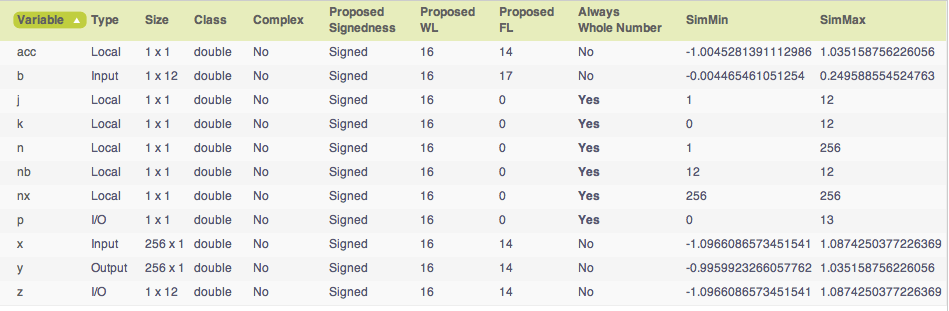
Use showInstrumentationResults to view the data types of all your variables and the minimum and maximum values that were logged during the test file run. Look at the maximum value logged for the output variable y and accumulator variable acc and note that they attained the theoretical maximum output value that you calculated previously.
showInstrumentationResults fir_filt_circ_buff_original_entry_point_mexTo see these results in the instrumented Code Generation Report:
Select function
fir_filt_circ_buff_originalSelect the Variables tab

Validate Original Function
Every time you modify your function, validate that the results still match your baseline.
fir_filt_circ_buff_plot2(2,titles,t,x,y0,y1)

Convert Functions to Use Types Tables
To separate data types from the algorithm, you:
Create a table of data type definitions.
Modify the algorithm code to use data types from that table.
This example shows the iterative steps by creating different files. In practice, you can make the iterative changes to the same file.
Original Types Table
Create a types table using a structure with prototypes for the variables set to their original types. Use the baseline types to validate that you made the initial conversion correctly, and also use it to programmatically toggle your function between floating-point and fixed-point types. The index variables j, k, n, nb, nx are automatically converted to integers by MATLAB Coder™, so you don't need to specify their types in the table.
Specify the prototype values as empty ([ ]) since the data types are used, but not the values.
function T = fir_filt_circ_buff_original_types()
    T.acc=double([]);
    T.b=double([]);
    T.p=double([]);
    T.x=double([]);
    T.y=double([]);
    T.z=double([]);
end
Type-Aware Filter Function
Prepare the filter function and entry-point function to be type-aware by using the cast and zeros functions and the types table.
Use subscripted assignment acc(:)=..., p(:)=1, and k(:)=nb to preserve data types during assignment. See the Cast fi Objects for more details about subscripted assignment and preserving data types.
The function call y = zeros(size(x),'like',T.y) creates an array of zeros the same size as x with the properties of variable T.y. Initially, T.y is a double defined in function fir_filt_circ_buff_original_types, but it is re-defined as a fixed-point type later in this example.
The function call acc = cast(0,'like',T.acc) casts the value 0 with the same properties as variable T.acc. Initially, T.acc is a double defined in function fir_filt_circ_buff_original_types, but it is re-defined as a fixed-point type later in this example.
function [y,z,p] = fir_filt_circ_buff_typed(b,x,z,p,T)
    y = zeros(size(x),'like',T.y);
    nx = length(x);
    nb = length(b);
    for n=1:nx
        p(:)=p+1; if p>nb, p(:)=1; end
        z(p) = x(n);
        acc = cast(0,'like',T.acc);
        k = p;
        for j=1:nb
            acc(:) = acc + b(j)*z(k);
            k(:)=k-1; if k<1, k(:)=nb; end
        end
        y(n) = acc;
    end
end
Type-Aware Entry-Point Function
The function call p1 = cast(0,'like',T1.p) casts the value 0 with the same properties as variable T1.p. Initially, T1.p is a double defined in function fir_filt_circ_buff_original_types, but it is re-defined as an integer type later in this example.
The function call z1 = zeros(size(b),'like',T1.z) creates an array of zeros the same size as b with the properties of variable T1.z. Initially, T1.z is a double defined in function fir_filt_circ_buff_original_types, but it is re-defined as a fixed-point type later in this example.
function y1 = fir_filt_circ_buff_typed_entry_point(b,x,reset)
   if nargin<3, reset = true; end
   %
   % Baseline types
   %
   T1 = fir_filt_circ_buff_original_types();
   % Each call to the filter needs to maintain its own states.
   persistent z1 p1
   if isempty(z1) || reset
       p1 = cast(0,'like',T1.p);
       z1 = zeros(size(b),'like',T1.z);
   end
   b1 = cast(b,'like',T1.b);
   x1 = cast(x,'like',T1.x);
   [y1,z1,p1] = fir_filt_circ_buff_typed(b1,x1,z1,p1,T1);
end
Validate Modified Function
Every time you modify your function, validate that the results still match your baseline. Since you used the original types in the types table, the outputs should be identical. This validates that you made the conversion to separate the types from the algorithm correctly.
buildInstrumentedMex fir_filt_circ_buff_typed_entry_point -args {b, x(:,1), reset}

y1 = fir_filt_circ_buff_typed_test(b,x);
fir_filt_circ_buff_plot2(3,titles,t,x,y0,y1)

Propose Data Types from Simulation Min/Max Logs
Use the showInstrumentationResults function to propose fixed-point fraction lengths, given a default signed fixed-point type and 16-bit word length.
showInstrumentationResults fir_filt_circ_buff_original_entry_point_mex ...
    -defaultDT numerictype(1,16) -proposeFL
In the instrumented Code Generation Report, select function fir_filt_circ_buff_original and the Variables tab to see these results.
Create a Fixed-Point Types Table
Use the proposed types from the Code Generation Report to guide you in choosing fixed-point types and create a fixed-point types table using a structure with prototypes for the variables.
Use your knowledge of the algorithm to improve on the proposals. For example, you are using the acc variable as an accumulator, so make it 32-bits. From the Code Generation Report, you can see that acc needs at least 2 integer bits to prevent overflow, so set the fraction length to 30.
Variable p is used as an index, so you can make it a builtin 16-bit integer.
Specify the prototype values as empty ([ ]) since the data types are used, but not the values.
function T = fir_filt_circ_buff_fixed_point_types()
    T.acc=fi([],true,32,30);
    T.b=fi([],true,16,17);
    T.p=int16([]);
    T.x=fi([],true,16,14);
    T.y=fi([],true,16,14);
    T.z=fi([],true,16,14);
end
Add Fixed Point to Entry-Point Function
Add a call to the fixed-point types table in the entry-point function:
T2 = fir_filt_circ_buff_fixed_point_types();
persistent z2 p2
if isempty(z2) || reset
    p2 = cast(0,'like',T2.p);
    z2 = zeros(size(b),'like',T2.z);
end
b2 = cast(b,'like',T2.b);
x2 = cast(x,'like',T2.x);
[y2,z2,p2] = fir_filt_circ_buff_typed(b2,x2,z2,p2,T2);
Build and Run Algorithm with Fixed-Point Data Types
buildInstrumentedMex fir_filt_circ_buff_typed_entry_point -args {b, x(:,1), reset}

[y1,y2] = fir_filt_circ_buff_typed_test(b,x);

showInstrumentationResults fir_filt_circ_buff_typed_entry_point_mex
To see these results in the instrumented Code Generation Report:
Select the entry-point function,
fir_filt_circ_buff_typed_entry_point.Select
fir_filt_circ_buff_typedin this line of code:
[y2,z2,p2] = fir_filt_circ_buff_typed(b2,x2,z2,p2,T2);
Select the Variables tab.

16-bit Word Length, Full Precision Math
Validate that the results are within an acceptable tolerance of your baseline.
fir_filt_circ_buff_plot2(4,titles,t,x,y1,y2);

Your algorithm has now been converted to fixed-point MATLAB code. If you also want to convert to C-code, then proceed to the next section.
Generate C-Code
This section describes how to generate efficient C-code from the fixed-point MATLAB code from the previous section.
Required Products
You need MATLAB Coder to generate C-code, and you need Embedded Coder® for the hardware implementation settings used in this example.
Algorithm Tuned for Most-Efficient C-Code
The output variable y is initialized to zeros, and then completely overwritten before it is used. Therefore, filling y with all zeros is unnecessary. You can use the coder.nullcopy function to declare a variable without actually filling it with values, which makes the code in this case more efficient. However, you have to be very careful when using coder.nullcopy because if you access an element of a variable before it is assigned, then you are accessing uninitialized memory and its contents are unpredictable.
A rule of thumb for when to use coder.nullcopy is when the initialization takes significant time compared to the rest of the algorithm. If you are not sure, then the safest thing to do is to not use it.
function [y,z,p] = fir_filt_circ_buff_typed_codegen(b,x,z,p,T)
    % Use coder.nullcopy only when you are certain that every value of
    % the variable is overwritten before it is used.
    y = coder.nullcopy(zeros(size(x),'like',T.y));
    nx = length(x);
    nb = length(b);
    for n=1:nx
        p(:)=p+1; if p>nb, p(:)=1; end
        z(p) = x(n);
        acc = cast(0,'like',T.acc);
        k = p;
        for j=1:nb
            acc(:) = acc + b(j)*z(k);
            k(:)=k-1; if k<1, k(:)=nb; end
        end
        y(n) = acc;
    end
end
Native C-Code Types
You can set the fixed-point math properties to match the native actions of C. This generates the most efficient C-code, but this example shows that it can create problems with overflow and produce less accurate results which are corrected in the next section. It doesn't always create problems, though, so it is worth trying first to see if you can get the cleanest possible C-code.
Set the fixed-point math properties to use floor rounding and wrap overflow because those are the default actions in C.
Set the fixed-point math properties of products and sums to match native C 32-bit integer types, and to keep the least significant bits (LSBs) of math operations.
Add these settings to a fixed-point types table.
function T = fir_filt_circ_buff_dsp_types()
    F = fimath('RoundingMethod','Floor',...
               'OverflowAction','Wrap',...
               'ProductMode','KeepLSB',...
               'ProductWordLength',32,...
               'SumMode','KeepLSB',...
               'SumWordLength',32);
    T.acc=fi([],true,32,30,F);
    T.p=int16([]);
    T.b=fi([],true,16,17,F);
    T.x=fi([],true,16,14,F);
    T.y=fi([],true,16,14,F);
    T.z=fi([],true,16,14,F);
end
Test the Native C-Code Types
Add a call to the types table in the entry-point function and run the test file.
[y1,y2,y3] = fir_filt_circ_buff_typed_test(b,x); %#ok<*ASGLU>In the second row of plots, you can see that the maximum output error is twice the size of the input, indicating that a value that should have been positive overflowed to negative. You can also see that the other outputs did not overflow. This is why it is important to have your test file exercise the full range of values in addition to other typical inputs.
fir_filt_circ_buff_plot2(5,titles,t,x,y1,y3);

Use Scaled Double Types to Find Overflows
Scaled double variables store their data in double-precision floating-point, so they carry out arithmetic in full range. They also retain their fixed-point settings, so they are able to report when a computation goes out of the range of the fixed-point type.
Change the data types to scaled double, and add these settings to a scaled-double types table.
function T = fir_filt_circ_buff_scaled_double_types()
    F = fimath('RoundingMethod','Floor',...
               'OverflowAction','Wrap',...
               'ProductMode','KeepLSB',...
               'ProductWordLength',32,...
               'SumMode','KeepLSB',...
               'SumWordLength',32);
    DT = 'ScaledDouble';
    T.acc=fi([],true,32,30,F,'DataType',DT);
    T.p=int16([]);
    T.b=fi([],true,16,17,F,'DataType',DT);
    T.x=fi([],true,16,14,F,'DataType',DT);
    T.y=fi([],true,16,14,F,'DataType',DT);
    T.z=fi([],true,16,14,F,'DataType',DT);
end
Add a call to the scaled-double types table to the entry-point function and run the test file.
[y1,y2,y3,y4] = fir_filt_circ_buff_typed_test(b,x); %#ok<*NASGU>Show the instrumentation results with the scaled-double types.
showInstrumentationResults fir_filt_circ_buff_typed_entry_point_mexTo see these results in the instrumented Code Generation Report:
Select the entry-point function,
fir_filt_circ_buff_typed_entry_point.Select
fir_filt_circ_buff_typed_codegenin this line of code:
[y4,z4,p4] = fir_filt_circ_buff_typed_codegen(b4,x4,z4,p4,T4);
Select the Variables tab.
Look at the variables in the table. None of the variables overflowed, which indicates that the overflow occurred as the result of an operation.
Hover over the operators in the report (
+,-,*,=).Hover over the
+in this line of MATLAB code in the instrumented Code Generation Report:
acc(:) = acc + b(j)*z(k);
The report shows that the sum overflowed:

The reason the sum overflowed is that a full-precision product for b(j)*z(k) produces a numerictype(true,32,31) because b has numerictype(true,16,17) and z has numerictype(true,16,14). The sum type is set to "keep least significant bits" (KeepLSB), so the sum has numerictype(true,32,31). However, 2 integer bits are necessary to store the minimum and maximum simulated values of -1.0045 and +1.035, respectively.
Adjust to Avoid the Overflow
Set the fraction length of b to 16 instead of 17 so that b(j)*z(k) is numerictype(true,32,30), and so the sum is also numerictype(true,32,30) following the KeepLSB rule for sums.
Leave all other settings the same, and set
T.b=fi([],true,16,16,F);
Then the sum in this line of MATLAB code no longer overflows:
acc(:) = acc + b(j)*z(k);
Run the test file with the new settings and plot the results.
[y1,y2,y3,y4,y5] = fir_filt_circ_buff_typed_test(b,x);
You can see that the overflow has been avoided. However, the plots show a bias and a larger error due to using C's natural floor rounding. If this bias is acceptable to you, then you can stop here and the generated C-code is very clean.
fir_filt_circ_buff_plot2(6,titles,t,x,y1,y5);

Eliminate the Bias
If the bias is not acceptable in your application, then change the rounding method to 'Nearest' to eliminate the bias. Rounding to nearest generates slightly more complicated C-code, but it may be necessary for you if you want to eliminate the bias and have a smaller error.
The final fixed-point types table with nearest rounding and adjusted coefficient fraction length is:
function T = fir_filt_circ_buff_dsp_nearest_types()
    F = fimath('RoundingMethod','Nearest',...
               'OverflowAction','Wrap',...
               'ProductMode','KeepLSB',...
               'ProductWordLength',32,...
               'SumMode','KeepLSB',...
               'SumWordLength',32);
    T.acc=fi([],true,32,30,F);
    T.p=int16([]);
    T.b=fi([],true,16,16,F);
    T.x=fi([],true,16,14,F);
    T.y=fi([],true,16,14,F);
    T.z=fi([],true,16,14,F);
end
Call this types table from the entry-point function and run and plot the output.
[y1,y2,y3,y4,y5,y6] = fir_filt_circ_buff_typed_test(b,x);
fir_filt_circ_buff_plot2(7,titles,t,x,y1,y6);

Run Code Generation Command
Run this build function to generate C-code. It is a best practice to create a build function so you can generate C-code for your core algorithm without the entry-point function or test file so the C-code for the core algorithm can be included in a larger project.
function fir_filt_circ_buff_build_function()
    %
    % Declare input arguments
    %
    T = fir_filt_circ_buff_dsp_nearest_types();
    b = zeros(1,12,'like',T.b);
    x = zeros(256,1,'like',T.x);
    z = zeros(size(b),'like',T.z);
    p = cast(0,'like',T.p);
    %
    % Code generation configuration
    %
    h = coder.config('lib');
    h.PurelyIntegerCode = true;
    h.SaturateOnIntegerOverflow = false;
    h.SupportNonFinite = false;
    h.HardwareImplementation.ProdBitPerShort = 8;
    h.HardwareImplementation.ProdBitPerInt = 16;
    h.HardwareImplementation.ProdBitPerLong = 32;
    %
    % Generate C-code
    %
    codegen fir_filt_circ_buff_typed_codegen -args {b,x,z,p,T} -config h -launchreport
end
Generated C-Code
Using these settings, MATLAB Coder generates the following C-code:
void fir_filt_circ_buff_typed_codegen(const int16_T b[12], const int16_T x[256],
  int16_T z[12], int16_T *p, int16_T y[256])
{
  int16_T n;
  int32_T acc;
  int16_T k;
  int16_T j;
  for (n = 0; n < 256; n++) {
    (*p)++;
    if (*p > 12) {
      *p = 1;
    }
    z[*p - 1] = x[n];
    acc = 0L;
    k = *p;
    for (j = 0; j < 12; j++) {
      acc += (int32_T)b[j] * z[k - 1];
      k--;
      if (k < 1) {
        k = 12;
      }
    }
    y[n] = (int16_T)((acc >> 16) + ((acc & 32768L) != 0L));
  }
}
Run the following code to restore the global states.
fipref(FIPREF_STATE);
clearInstrumentationResults fir_filt_circ_buff_original_entry_point_mex
clearInstrumentationResults fir_filt_circ_buff_typed_entry_point_mex
clear fir_filt_circ_buff_original_entry_point_mex
clear fir_filt_circ_buff_typed_entry_point_mex
References:
[1] J. R. Ragazzini and L. A. Zadeh. "The analysis of sampled-data systems". In: Transactions of the American Institute of Electrical Engineers 71 (II) (1952), pp. 225–234.
You can also select a web site from the following list:
Americas
- América Latina (Español)
- Canada (English)
- United States (English)
Europe
- Belgium (English)
- Denmark (English)
- Deutschland (Deutsch)
- España (Español)
- Finland (English)
- France (Français)
- Ireland (English)
- Italia (Italiano)
- Luxembourg (English)
- Netherlands (English)
- Norway (English)
- Österreich (Deutsch)
- Portugal (English)
- Sweden (English)
- Switzerland
- United Kingdom (English)