initvisionbboxkf

Create constant-velocity linear Kalman filter for 2-D axis-aligned bounding box from detection report

Since R2024a

Syntax

filter = initvisionbboxkf(detection)

filter = initvisionbboxkf(detection,Name=Value)

Description

filter = initvisionbboxkf(detection) creates and initializes a constant-velocity linear Kalman filter for a 2-D axis-aligned bounding box from information contained in a detection report. For more details, see trackingKF.

filter = initvisionbboxkf(detection,Name=Value) specifies filter properties using one or more name-value arguments. Unspecified properties have default values. For example, filter = initvisionbboxkf(detection,FrameRate=45) creates a Kalman filter object with a frame rate of 45 frames per second.

Examples

Create Constant-Velocity Linear Kalman Filter Using Bounding Box

Create a constant-velocity linear Kalman filter object, trackingKF, based on a 2-D bounding box, from a tracking video containing an initial detection report.

Initialize Kalman Filter

Define a bounding box with its lower left corner located at (200, 400), a width of 100 pixels and a height of 120 pixels. Create an objectDetection object based on this bounding box at the first frame.

bbox = [200 400 100 120]; % [x y width height]
detection = objectDetection(0,bbox);

Specify the frame rate of the tracking video as 20 frames per second and the frame size as 800 by 600 pixels. Create and initialize a trackingKF object using the detection object, frame rate, and resolution.

framerate = 20;
framesize = [800 600];
filter = initvisionbboxkf(detection,FrameRate=framerate,FrameSize=framesize)

filter = 
  trackingKF with properties:

                   State: [8x1 double]
         StateCovariance: [8x8 double]

             MotionModel: 'Custom'
    StateTransitionModel: [8x8 double]
            ControlModel: []
            ProcessNoise: [8x8 double]

        MeasurementModel: [4x8 double]
        MeasurementNoise: [4x4 double]

         MaxNumOOSMSteps: 0

         EnableSmoothing: 0

Predict and Correct Next State

Create a new bounding box, bbox2, at the second frame. Its lower left corner is located at (245, 275) while its width increases to 130 pixels and its height increases to 160 pixels.

bbox2 = [245 275 130 160];

Predict the filter state of the second frame and correct it using bbox2. For more information about state prediction and correction, see objectDetection.

estimatedState2 = predict(filter);
correctedState2 = correct(filter,bbox2);

Predict and display the filter state of the third frame.

estimatedState3 = predict(filter) % [x vx y vy w vw h vh]'

estimatedState3 = 8×1

  235.1562
  178.1250
  302.3438
 -494.7917
  123.4375
  118.7500
  151.2500
  158.3333

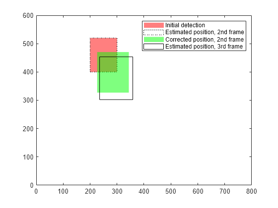
Plot the initial bounding box, the corrected bounding box position for the second frame, and the estimated bounding box positions for the second and third frames in the same figure. The estimated position for the second frame overlaps with the initial detection because the velocity of the initialized filter is null by default.

figure
xlim([0 framesize(1)])
ylim([0 framesize(2)])
hold on
box on
targetplot(detection.Measurement,"r","none",0.5)
targetplot(estimatedState2,"w",":",0)
targetplot(correctedState2,"g","none",0.5)
targetplot(estimatedState3,"w","-",0)
legend(["Initial detection" "Estimated position, 2nd frame" "Corrected position, 2nd frame" "Estimated position, 3rd frame"])

function targetplot(state,fc,ls,fa)
if length(state)>4
    X=[state(1),state(1),state(1)+state(5),state(1)+state(5)];
    Y=[state(3),state(3)+state(7),state(3)+state(7),state(3)];
else
    X=[state(1),state(1),state(1)+state(3),state(1)+state(3)];
    Y=[state(2),state(2)+state(4),state(2)+state(4),state(2)];
end
patch(XData=X,YData=Y,FaceColor=fc,LineStyle=ls,FaceAlpha=fa);
end 

Input Arguments

detection — Detection report

objectDetection object | structure

Detection report, specified as an objectDetection object or a structure with fields Measurement and MeasurementNoise. Measurement must contain a four-element bounding box vector [x y w h] specified in pixels, where

• x and y are the coordinates of a point on the bounding box in the image frame. Select this point from anywhere on the bounding box, such as a corner or the center. However, the selected point must remain consistent throughout the tracking process.

• w is the width of the bounding box.

• h is the height of the bounding box.

MeasurementNoise is a 4-by-4 matrix containing measurement noise covariances corresponding to the Measurement elements. If the detection report is a structure, you must specify MeasurementNoise manually. If the detection report is an objectDetection object, and if you do not specify the MeasurementNoise matrix, MeasurementNoise defaults to an identity matrix.

Example: objectDetection(0,[200 400 50 60],MeasurementNoise=diag([0.1 0.2 0.1 0.2]))

Example: detection.Measurement = [200 400 50 60]; detection.MeasurementNoise = diag([0.1 0.2 0.1 0.2])

Name-Value Arguments

Specify optional pairs of arguments as Name1=Value1,...,NameN=ValueN, where Name is the argument name and Value is the corresponding value. Name-value arguments must appear after other arguments, but the order of the pairs does not matter.

Example: filter = initvisionbboxkf(detection,FrameSize = [1280 720])

FrameRate — Tracking frame rate

30 (default) | positive numeric scalar

Tracking frame rate in frames per second, specified as a positive numeric scalar.

Data Types: single | double | int8 | int16 | int32 | int64 | uint8 | uint16 | uint32 | uint64

FrameSize — Tracking frame size

[1920 1080] (default) | [width height]

Tracking frame size in pixels, specified as a row or column vector of the form [width height].

Data Types: single | double | int8 | int16 | int32 | int64 | uint8 | uint16 | uint32 | uint64

NoiseIntensity — Process noise intensities

[1e-2 1e-2 1e-2 1e-2] (default) | [qx qy qw qh]

Process noise intensities of the constant velocity model, specified as a four-element row or column vector of noise intensities [qx qy qw qh] corresponding to each element of the bounding box.

Output Arguments

filter — Constant-velocity linear Kalman filter for 2-D axis-aligned bounding box

trackingKF object

Constant-velocity Kalman filter for 2-D axis-aligned bounding box, returned as a trackingKF object. You can determine the state of this Kalman filter object by using filter.State = [x vx y vy w vw h vh]', where [x y w h] are the coordinates, width, height of the bounding box, and [vx vy vw vh] are their corresponding time derivatives.

Algorithms

• You can use initvisionbboxkf as the FilterInitializationFcn property of the trackerGNN, trackerJPDA, and trackerTOMHT System objects.

• When using this function to initialize a trackingKF object, it employs a 1-D constant-velocity model with additive process noise. This model updates the system state for each bounding box element, p, and its time derivative, v using the following equation:

  $$\left[\begin{array}{c}p(k+1)\\ v(k+1)\end{array}\right]=\left[\begin{array}{cc}1& T\\ 0& 1\end{array}\right]\left[\begin{array}{c}p(k)\\ v(k)\end{array}\right]+w(k),$$

  where T is the inverse of the FrameRate, the process noise w(k) has a covariance:

  $$\text{cov}\left(w(k)\right)=q\left[\begin{array}{cc}\frac{T^3}{3}& \frac{T^2}{2}\\ \frac{T^2}{2}& T\end{array}\right],$$

  which can be written after normalization as

  $$\text{cov}\left(w(k)\right)={\left({\gamma }^{p,v}\right)}^{2}G\left(q^{p,v}{I}_2\right)G\text{'}.$$

  The scaling factor γ equals the minimum value of the frame size. You can adjust the unitless, time-independent noise intensity, q^p,v, by using the NoiseIntensity input argument. G is the lower-triangular Cholesky factor of the noise covariance, as returned by the chol function when triangle is set to 'lower'. G' is the transpose of G.

  $$G=\text{Chol}\left(\left[\begin{array}{cc}\frac{T^3}{3}& \frac{T^2}{2}\\ \frac{T^2}{2}& T\end{array}\right]\right)=\left[\begin{array}{cc}\frac{\sqrt{T^3}}{\sqrt{3}}& 0\\ \frac{\sqrt{3T}}{2}& \frac{\sqrt{T}}{2}\end{array}\right]$$

References

[1] J. Krejčí, O. Kost, O. Straka, and J. Duník, "Bounding Box Dynamics in Visual Tracking: Modeling and Noise Covariance Estimation," 2023 26th International Conference on Information Fusion (FUSION), IEEE, 2023, pp. 1–6.

Extended Capabilities

C/C++ Code Generation
Generate C and C++ code using MATLAB® Coder™.

Version History

Introduced in R2024a