Interpret surrogateoptplot
R2026bThe surrogateoptplot plot function provides a good deal of information about the surrogate optimization steps.
Minimize Bounded Function
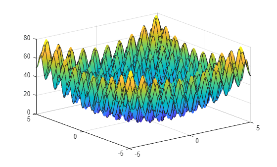
For example, consider the plot of the steps surrogateopt takes on the test function rastriginsfcn, which is available when you run this example. This function has a global minimum value of 0 at the point [0,0].
Create a surface plot of rastriginsfcn.
fsurf(@(x,y)reshape(rastriginsfcn([x(:),y(:)]),size(x)));
Plot Minimization Process
By giving asymmetric bounds, you encourage surrogateopt to search away from the global minimum. Set asymmetric bounds of [-3,-3] and [9,10]. Set options to use the surrogateoptplot plot function, and then call surrogateopt.
lb = [-3,-3];
ub = [9,10];
options = optimoptions("surrogateopt",PlotFcn="surrogateoptplot");
rng(100)
[x,fval] = surrogateopt(@rastriginsfcn,lb,ub,options);
surrogateopt stopped because it exceeded the function evaluation limit set by
'options.MaxFunctionEvaluations'.
Interpret Plot
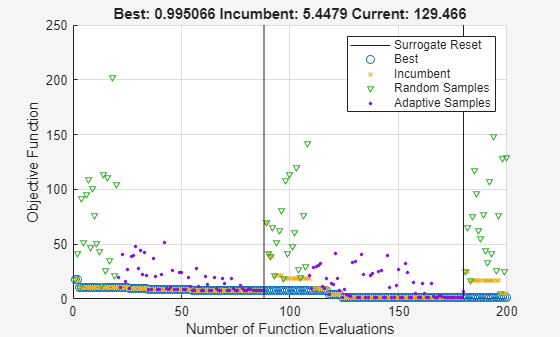
Begin interpreting the plot from its left side. For details of the algorithm steps, see Surrogate Optimization Algorithm.
The first points are colored triangles, indicating quasirandom samples of the function within the problem bounds. These points, labeled "Random Samples" in the legend, come from the Construct Surrogate phase.
Next are dots indicating the adaptive points, the points created in the Search for Minimum phase. These points are labeled "Adaptive Samples" in the legend.
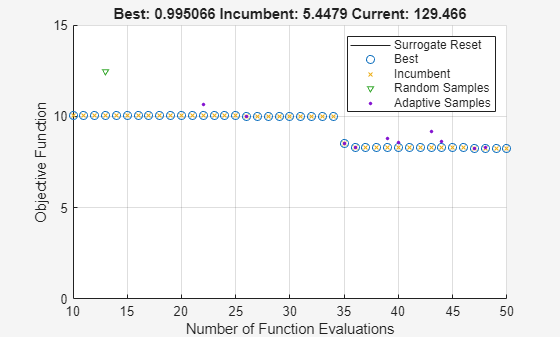
The circles (overlapping to look like a thick line) represent the best (lowest) objective function value found. These points are labeled "Best" in the legend. Shortly after evaluation number 30,
surrogateoptis stuck in a local minimum with an objective function value near 8. Zoom in to see this behavior more clearly.
xlim([10 50])
ylim([0 15])
Near evaluation number 90, a vertical line indicates a surrogate reset. At this point, the algorithm returns to the Construct Surrogate phase.
The colored x points represent the incumbent, which are the best points found since the previous surrogate reset.
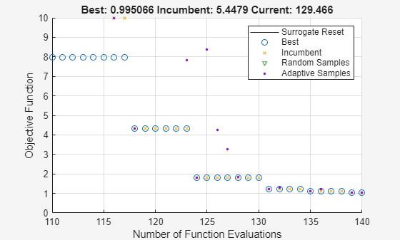
After evaluation number 115, the incumbent improves on the previous best point a few times, attaining a value of about 1. Zoom in to see this behavior more clearly.
xlim([110 140])
ylim([0 10])
The solver has another surrogate reset near evaluation 180.
The optimization halts at evaluation number 200 because it is the default function evaluation limit for a 2-D problem.
Problem with Nonlinear and Integer Constraints
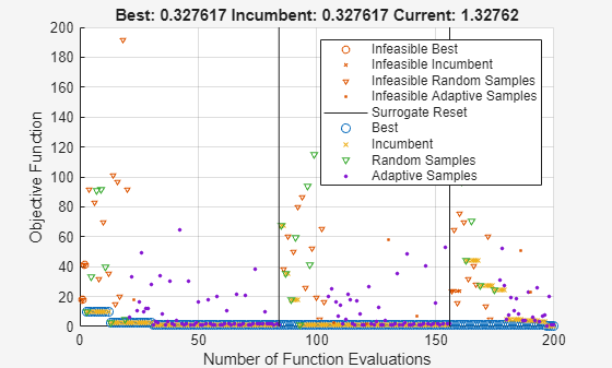
The surrogateoptplot display changes when you have nonlinear constraints. Impose the constraint that x(1) is integer-valued, and the nonlinear constraint that . For the function that implements this constraint, see rasfcn at the end of this example.
fun = @rasfcn;
Set integer constraints by setting intcon = 1, and run the minimization.
intcon = 1;
[x,fval] = surrogateopt(fun,lb,ub,intcon,options);
surrogateopt stopped because it exceeded the function evaluation limit set by
'options.MaxFunctionEvaluations'.
The plot now shows colored markers where surrogateopt evaluates infeasible points. The final point is close to the true minimum point of [0,0].
disp(x)
0 0.0407
The integer constraint likely helps surrogateopt find the true minimum by reducing the search space.
function F = rasfcn(x)
F.Fval = rastriginsfcn(x);
F.Ineq = x(1)^2 - 2 - x(2);
end

