pzmap
Pole-zero map of dynamic system
Syntax
Description
[
returns the system poles and transmission zeros of the dynamic
system model
p,z] = pzmap(sys)sys.
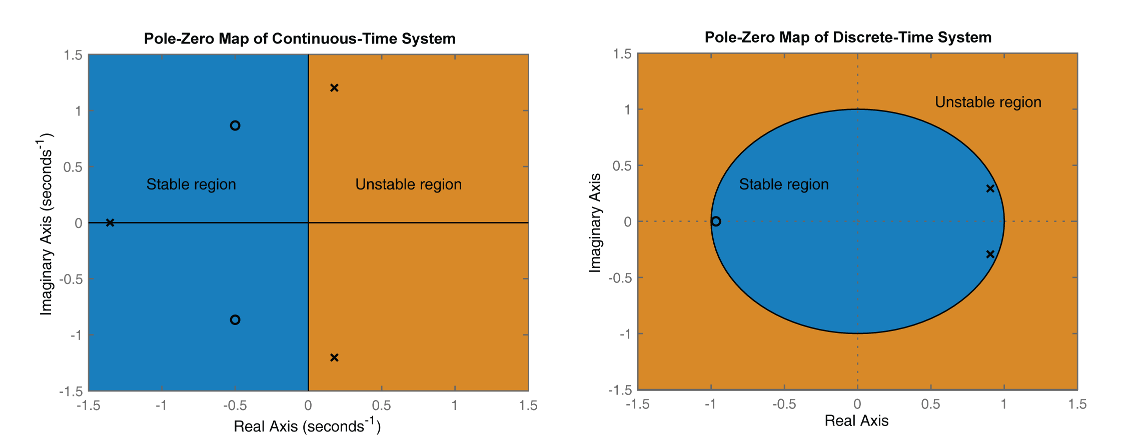
The following figure shows pole-zero maps for a continuous-time (left) and discrete-time (right) linear time-variant model.
In continuous-time systems, all the poles on the complex s-plane must be in the left-half plane (blue region) to ensure stability. The system is marginally stable if distinct poles lie on the imaginary axis, that is, the real parts of the poles are zero.
In discrete-time systems, all the poles in the complex z-plane must lie inside the unit circle (blue region). The system is marginally stable if it has one or more poles lying on the unit circle.
pzmap( plots a pole-zero map for
sys)sys. In the plot, x and
o represent poles and zeros, respectively. For SISO
systems, pzmap plots the system poles and zeros. For MIMO
systems, pzmap plots the system poles and transmission
zeros.
Examples
Plot the poles and zeros of the continuous-time system represented by the following transfer function:
H = tf([2 5 1],[1 3 5]);
pzmap(H)
grid on
Turning on the grid displays lines of constant damping ratio (zeta) and lines of constant natural frequency (wn). This system has two real zeros, marked by o on the plot. The system also has a pair of complex poles, marked by x.
Plot the pole-zero map of a discrete time identified state-space (idss) model. In practice you can obtain an idss model by estimation based on input-output measurements of a system. For this example, create one from state-space data.
A = [0.1 0; 0.2 -0.9];
B = [.1 ; 0.1];
C = [10 5];
D = [0];
sys = idss(A,B,C,D,'Ts',0.1);
Examine the pole-zero map.
pzmap(sys)

System poles are marked by x, and zeros are marked by o.
For this example, load a 3-by-1 array of transfer function models.
load("tfArray.mat","sys");
size(sys)
3x1 array of transfer functions.
Each model has 1 outputs and 1 inputs.
Plot the poles and zeros of each model in the array with distinct colors. For this example, use red for the first model, green for the second and blue for the third model in the array.
pzplot(sys(:,:,1),"r",sys(:,:,2),"g",sys(:,:,3),"b")
grid

The grid shows lines of constant damping ratio and natural frequency in the s-plane of the pole-zero plot.
Use pzmap to calculate the poles and zeros of the following transfer function:
sys = tf([4.2,0.25,-0.004],[1,9.6,17]);
[p,z] = pzmap(sys)
p = 2×1

   -7.2576
   -2.3424
z = 2×1

   -0.0726
    0.0131
This example uses a model of a building with eight floors, each with three degrees of freedom: two displacements and one rotation. The I/O relationship for any one of these displacements is represented as a 48-state model, where each state represents a displacement or its rate of change (velocity).
Load the building model.
load('building.mat');
size(G)
State-space model with 1 outputs, 1 inputs, and 48 states.
Plot the poles and zeros of the system.
pzmap(G)

From the plot, observe that there are numerous near-canceling pole-zero pairs that could be potentially eliminated to simplify the model, with no effect on the overall model response. pzmap is useful to visually identify such near-canceling pole-zero pairs to perform pole-zero simplification.
Input Arguments
Output Arguments
Tips
For MIMO models,
pzmapdisplays all system poles and transmission zeros on a single plot. To map poles and zeros for individual input-output pairs, useiopzmap.For additional options to customize the appearance of the pole-zero plot, use
pzplot.Plots created using
pzmapdo not support multiline titles or labels specified as string arrays or cell arrays of character vectors. To specify multiline titles and labels, use a single string with anewlinecharacter.pzmap(sys,u,t) title("first line" + newline + "second line");