tf
Transfer function model
Description
Use tf to create real-valued or complex-valued transfer
function models, or to convert dynamic system
models to transfer function form.
Transfer functions are a frequency-domain representation of linear time-invariant
systems. For instance, consider a continuous-time SISO dynamic system represented by the
transfer function sys(s) = N(s)/D(s), where s = jw
and N(s) and D(s) are called the numerator and
denominator polynomials, respectively. The tf model object can
represent SISO or MIMO transfer functions in continuous time or discrete time.
You can create a transfer function model object either by specifying its coefficients
directly, or by converting a model of another type (such as a state-space model
ss) to transfer-function form. For more information, see Transfer Functions.
You can also use tf to create generalized state-space (genss) models or uncertain state-space (uss (Robust Control Toolbox)) models.
Creation
Syntax
Description
Create Transfer Function Model
sys = tf(numerator,denominator)Numerator and Denominator
properties. For instance, consider a continuous-time SISO dynamic system
represented by the transfer function sys(s) = N(s)/D(s),
the input arguments numerator and
denominator are the coefficients of
N(s) and D(s),
respectively.
sys = tf(numerator,denominator,ts)Numerator, Denominator, and
Ts properties. For instance, consider a
discrete-time SISO dynamic system represented by the transfer function
sys(z) = N(z)/D(z), the input arguments
numerator and denominator are
the coefficients of N(z) and D(z),
respectively. To leave the sample time unspecified, set
ts input argument to -1.
sys = tf(numerator,denominator,ltiSys)ltiSys, including the sample time.
sys = tf(___,PropertyName=Value)
Convert To Transfer Function Model
sys = tf(ltiSys,Name=Value)ltiSys by computing zeros and poles based on one or
more specified name-value arguments. Because this method calculates zeros
for each input-output pair, it is most suitable for models with small
input-output sizes. (since R2025a)
Create Variable for Rational Expression
s = tf('s') creates special variable
s that you can use in a rational expression to create
a continuous-time transfer function model. Using a rational expression can
sometimes be easier and more intuitive than specifying polynomial
coefficients.
Input Arguments
Name-Value Arguments
Output Arguments
Properties
Object Functions
The following lists contain a representative subset of the functions you can use with
tf models. In general, any function applicable to Dynamic System Models
is applicable to a tf object.
Examples
For this example, consider the following SISO transfer function model:
Specify the numerator and denominator coefficients ordered in descending powers of s, and create the transfer function model.
numerator = 1;
denominator = [2,3,4];
sys = tf(numerator,denominator)
sys =

         1
  ---------------
  2 s^2 + 3 s + 4

Continuous-time transfer function.
Model Properties
For this example, consider the following discrete-time SISO transfer function model:
Specify the numerator and denominator coefficients ordered in descending powers of z and the sample time of 0.1 seconds. Create the discrete-time transfer function model.
numerator = [2,0];
denominator = [4,0,3,-1];
ts = 0.1;
sys = tf(numerator,denominator,ts)
sys =

        2 z
  ---------------
  4 z^3 + 3 z - 1

Sample time: 0.1 seconds
Discrete-time transfer function.
Model Properties
For this example, consider a transfer function model that represents a second-order system with known natural frequency and damping ratio.
The transfer function of a second-order system, expressed in terms of its damping ratio and natural frequency , is:
Assuming a damping ratio, = 0.25 and natural frequency, = 3 rad/s, create the second order transfer function.
zeta = 0.25;
w0 = 3;
numerator = w0^2;
denominator = [1,2*zeta*w0,w0^2];
sys = tf(numerator,denominator)
sys =

         9
  ---------------
  s^2 + 1.5 s + 9

Continuous-time transfer function.
Model Properties
Examine the response of this transfer function to a step input.
stepplot(sys)

The plot shows the ringdown expected of a second-order system with a low damping ratio.
Create a transfer function for the discrete-time, multi-input, multi-output model:
with sample time ts = 0.2 seconds.
Specify the numerator coefficients as a 2-by-2 matrix.
numerators = {1 [1 0];[-1 2] 3};Specify the coefficients of the common denominator as a row vector.
denominator = [1 0.3];
Create the discrete-time MIMO transfer function model.
ts = 0.2;
sys = tf(numerators,denominator,ts)
sys =

  From input 1 to output...
          1
   1:  -------
       z + 0.3

       -z + 2
   2:  -------
       z + 0.3

  From input 2 to output...
          z
   1:  -------
       z + 0.3

          3
   2:  -------
       z + 0.3

Sample time: 0.2 seconds
Discrete-time transfer function.
Model Properties
For more information on creating MIMO transfer functions, see MIMO Transfer Functions.
In this example, you create a MIMO transfer function model by concatenating SISO transfer function models. Consider the following single-input, two-output transfer function:
Specify the MIMO transfer function model by concatenating the SISO entries.
sys1 = tf([1 -1],[1 1]);
sys2 = tf([1 2],[1 4 5]);
sys = [sys1;sys2]
sys =

  From input to output...
       s - 1
   1:  -----
       s + 1

           s + 2
   2:  -------------
       s^2 + 4 s + 5

Continuous-time transfer function.
Model Properties
For more information on creating MIMO transfer functions, see MIMO Transfer Functions.
For this example, create a continuous-time transfer function model using rational expressions. Using a rational expression can sometimes be easier and more intuitive than specifying polynomial coefficients of the numerator and denominator.
Consider the following system:
To create the transfer function model, first specify s as a tf object.
s = tf('s')s = s Continuous-time transfer function. Model Properties
Create the transfer function model using s in the rational expression.
sys = s/(s^2 + 2*s + 10)
sys =

        s
  --------------
  s^2 + 2 s + 10

Continuous-time transfer function.
Model Properties
For this example, create a discrete-time transfer function model using a rational expression. Using a rational expression can sometimes be easier and more intuitive than specifying polynomial coefficients.
Consider the following system:
To create the transfer function model, first specify z as a tf object and the sample time Ts.
ts = 0.1;
z = tf('z',ts)
z = z Sample time: 0.1 seconds Discrete-time transfer function. Model Properties
Create the transfer function model using z in the rational expression.
sys = (z - 1) / (z^2 - 1.85*z + 0.9)
sys =

        z - 1
  ------------------
  z^2 - 1.85 z + 0.9

Sample time: 0.1 seconds
Discrete-time transfer function.
Model Properties
For this example, create a transfer function model with properties inherited from another transfer function model. Consider the following two transfer functions:
For this example, create sys1 with the TimeUnit and InputDelay property set to 'minutes'.
numerator1 = [2,0];
denominator1 = [1,8,0];
sys1 = tf(numerator1,denominator1,'TimeUnit','minutes','InputUnit','minutes')
sys1 =

     2 s
  ---------
  s^2 + 8 s

Continuous-time transfer function.
Model Properties
propValues1 = [sys1.TimeUnit,sys1.InputUnit]
propValues1 = 1×2 cell
    {'minutes'}    {'minutes'}
Create the second transfer function model with properties inherited from sys1.
numerator2 = [1,-1];
denominator2 = [7,2,0,0,9];
sys2 = tf(numerator2,denominator2,sys1)
sys2 =

        s - 1
  -----------------
  7 s^4 + 2 s^3 + 9

Continuous-time transfer function.
Model Properties
propValues2 = [sys2.TimeUnit,sys2.InputUnit]
propValues2 = 1×2 cell
    {'minutes'}    {'minutes'}
Observe that the transfer function model sys2 has that same properties as sys1.
You can use a for loop to specify an array of transfer function models.
First, pre-allocate the transfer function array with zeros.
sys = tf(zeros(1,1,3));
The first two indices represent the number of outputs and inputs for the models, while the third index is the number of models in the array.
Create the transfer function model array using a rational expression in the for loop.
s = tf('s');
for k = 1:3
    sys(:,:,k) = k/(s^2+s+k);
end
sys
sys(:,:,1,1) =

       1
  -----------
  s^2 + s + 1


sys(:,:,2,1) =

       2
  -----------
  s^2 + s + 2


sys(:,:,3,1) =

       3
  -----------
  s^2 + s + 3

3x1 array of continuous-time transfer functions.
Model Properties
For this example, compute the transfer function of the following state-space model:
Create the state-space model using the state-space matrices.
A = [-2 -1;1 -2];
B = [1 1;2 -1];
C = [1 0];
D = [0 1];
ltiSys = ss(A,B,C,D);
Convert the state-space model ltiSys to a transfer function.
sys = tf(ltiSys)
sys =

  From input 1 to output:
        s
  -------------
  s^2 + 4 s + 5

  From input 2 to output:
  s^2 + 5 s + 8
  -------------
  s^2 + 4 s + 5

Continuous-time transfer function.
Model Properties
For this example, extract the measured and noise components of an identified polynomial model into two separate transfer functions.
Load the Box-Jenkins polynomial model ltiSys in identifiedModel.mat.
load('identifiedModel.mat','ltiSys');
ltiSys is an identified discrete-time model of the form: , where represents the measured component and the noise component.
Extract the measured and noise components as transfer functions.
sysMeas = tf(ltiSys,'measured') sysMeas =
From input "u1" to output "y1":
-0.1426 z^-1 + 0.1958 z^-2
z^(-2) * ----------------------------
1 - 1.575 z^-1 + 0.6115 z^-2
Sample time: 0.04 seconds
Discrete-time transfer function.
Model Properties
sysNoise = tf(ltiSys,'noise')sysNoise =
From input "v@y1" to output "y1":
0.04556 + 0.03301 z^-1
----------------------------------------
1 - 1.026 z^-1 + 0.26 z^-2 - 0.1949 z^-3
Input groups:
Name Channels
Noise 1
Sample time: 0.04 seconds
Discrete-time transfer function.
Model Properties
The measured component can serve as a plant model, while the noise component can be used as a disturbance model for control system design.
Transfer function model objects include model data that helps you keep track of what the model represents. For instance, you can assign names to the inputs and outputs of your model.
Consider the following continuous-time MIMO transfer function model:
The model has one input Current, and two outputs Torque and Angular velocity.
First, specify the numerator and denominator coefficients of the model.
numerators = {[1 1] ; 1};
denominators = {[1 2 2] ; [1 0]};
Create the transfer function model, specifying the input name and output names.
sys = tf(numerators,denominators,'InputName','Current',...
        'OutputName',{'Torque' 'Angular Velocity'})
sys =

  From input "Current" to output...
                s + 1
   Torque:  -------------
            s^2 + 2 s + 2

                      1
   Angular Velocity:  -
                      s

Continuous-time transfer function.
Model Properties
For this example, specify polynomial ordering in discrete-time transfer function models using the 'Variable' property.
Consider the following discrete-time transfer functions with sample time 0.1 seconds:
Create the first discrete-time transfer function by specifying the z coefficients.
numerator = [1,0,0];
denominator = [1,2,3];
ts = 0.1;
sys1 = tf(numerator,denominator,ts)
sys1 =

       z^2
  -------------
  z^2 + 2 z + 3

Sample time: 0.1 seconds
Discrete-time transfer function.
Model Properties
The coefficients of sys1 are ordered in descending powers of z.
tf switches convention based on the value of the 'Variable' property. Since sys2 is the inverse transfer function model of sys1, specify 'Variable' as 'z^-1' and use the same numerator and denominator coefficients.
sys2 = tf(numerator,denominator,ts,'Variable','z^-1')
sys2 =

           1
  -------------------
  1 + 2 z^-1 + 3 z^-2

Sample time: 0.1 seconds
Discrete-time transfer function.
Model Properties
The coefficients of sys2 are now ordered in ascending powers of z^-1.
Based on different conventions, you can specify polynomial ordering in transfer function models using the 'Variable' property.
In this example, you will create a low-pass filter with one tunable parameter a:
Since the numerator and denominator coefficients of a tunableTF block are independent, you cannot use tunableTF to represent F. Instead, construct F using the tunable real parameter object realp.
Create a real tunable parameter with an initial value of 10.
a = realp('a',10)a =
Name: 'a'
Value: 10
Minimum: -Inf
Maximum: Inf
Free: 1
Real scalar parameter.
Use tf to create the tunable low-pass filter F.
numerator = a;
denominator = [1,a];
F = tf(numerator,denominator)
Generalized continuous-time state-space model with 1 outputs, 1 inputs, 1 states, and the following blocks:
  a: Scalar parameter, 2 occurrences.
Model Properties

Type "ss(F)" to see the current value and "F.Blocks" to interact with the blocks.
F is a genss object which has the tunable parameter a in its Blocks property. You can connect F with other tunable or numeric models to create more complex control system models. For an example, see Control System with Tunable Components.
In this example, you will create a static gain MIMO transfer function model.
Consider the following two-input, two-output static gain matrix m:
Specify the gain matrix and create the static gain transfer function model.
m = [2,4;...
    3,5];
sys1 = tf(m)
sys1 = From input 1 to output... 1: 2 2: 3 From input 2 to output... 1: 4 2: 5 Static gain. Model Properties
You can use static gain transfer function model sys1 obtained above to cascade it with another transfer function model.
For this example, create another two-input, two-output discrete transfer function model and use the series function to connect the two models.
numerators = {1,[1,0];[-1,2],3};
denominator = [1,0.3];
ts = 0.2;
sys2 = tf(numerators,denominator,ts)
sys2 =
From input 1 to output...
1
1: -------
z + 0.3
-z + 2
2: -------
z + 0.3
From input 2 to output...
z
1: -------
z + 0.3
3
2: -------
z + 0.3
Sample time: 0.2 seconds
Discrete-time transfer function.
Model Properties
sys = series(sys1,sys2)
sys =

  From input 1 to output...
       3 z^2 + 2.9 z + 0.6
   1:  -------------------
       z^2 + 0.6 z + 0.09

       -2 z^2 + 12.4 z + 3.9
   2:  ---------------------
        z^2 + 0.6 z + 0.09

  From input 2 to output...
       5 z^2 + 5.5 z + 1.2
   1:  -------------------
       z^2 + 0.6 z + 0.09

       -4 z^2 + 21.8 z + 6.9
   2:  ---------------------
        z^2 + 0.6 z + 0.09

Sample time: 0.2 seconds
Discrete-time transfer function.
Model Properties
Since R2025a
This example shows how to obtain a truncated transfer function model of a sparse state-space model. This example uses a sparse model obtained from linearizing a thermal model of heat distribution in a circular cylindrical rod.
Load the model data.
load cylindricalRod.mat
sys = sparss(A,B,C,D,E);
w = logspace(-7,-1,20);
size(sys)
Sparse state-space model with 3 outputs, 1 inputs, and 7522 states.
Analyze the frequency response of the model.
sigmaplot(sys,w)

To obtain a truncated approximation, use tf and specify the frequency band of focus. For this model, you can use a frequency range from 0 rad/s to 0.01 rad/s to obtain the low-order approximation.
tsys = tf(sys,Focus=[0 1e-2],Display="off");Compare the frequency response.
sigmaplot(sys,tsys,w)
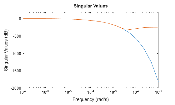
This thermal model has a very steep roll-off beyond 0.001 rad/s. By default, the reduced model obtained using tf does not provide a good match for this roll-off. To mitigate this, you can use the RollOff argument of tf and specify a minimum roll-off value beyond the frequency band of focus. Specify a roll-off slope value of -45, which corresponds to a rate of at least –900 db/decade.
tsys2 = tf(sys,Focus=[0 1e-2],RollOff=-45,Display="off");
sigmaplot(sys,tsys2,w)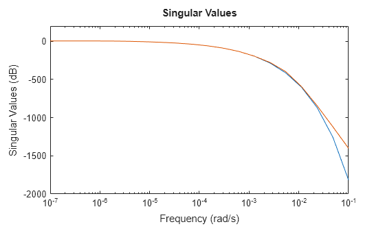
The reduced model now provides a much better approximation of the roll-off value. However, in this example, readjusting roll-off slope using tf requires recomputing zeros and poles. This may be computationally expensive in case of large-scale models. As an alternative, you can use the zero-pole truncation method of reducespec and adjust roll-off at no extra computation cost, after the software has computed poles and zeros. For an example, see Zero-Pole Truncation of Thermal Model.
Limitations
Transfer function models are ill-suited for numerical computations. Once created, convert them to state-space form before combining them with other models or performing model transformations. You can then convert the resulting models back to transfer function form for inspection purposes
An identified nonlinear model cannot be directly converted into a transfer function model using
tf. To obtain a transfer function model:Convert the nonlinear identified model to an identified LTI model using
linapp(System Identification Toolbox),idnlarx/linearize(System Identification Toolbox), oridnlhw/linearize(System Identification Toolbox).Then, convert the resulting model to a transfer function model using
tf.
Algorithms
To convert sparse models, tf uses the Krylov--Schur algorithm [1] for
inverse power iterations to compute poles and zeros in the specified frequency
band.
References
[1] Stewart, G. W. “A Krylov--Schur Algorithm for Large Eigenproblems.” SIAM Journal on Matrix Analysis and Applications 23, no. 3 (January 2002): 601–14. https://doi.org/10.1137/S0895479800371529.