usamap
Create axesm-based map for United States of America
Syntax
Description
usamap andstate
usamap( create an empty
state)axesm-based map (previously referred to as map axes)
with a Lambert Conformal Conic projection and map limits covering a US state or
group of states specified by state. The
axesm-based map is created in the current axes and the
axis limits are set tight around the map frame.
usamap 'conus' and
usamap('conus') create an empty
axesm-based map for the conterminous 48 states (that
is, all states excluding Alaska and Hawaii).
usamap with no arguments presents a menu from which you
can select a single state, the District of Columbia, the conterminous 48 states,
or all states.
h = usamap(___)axesm-based map.
h = usamap('all')axesm-based maps, inset within a single figure, for
the conterminous states, Alaska, and Hawaii, with a spherical Earth model and
other projection parameters suggested by the U.S. Geological Survey. The maps in
the three axes are shown at approximately the same scale. The handles for the
three axesm-based maps are returned in
h.
usamap('allequal') is the same as
usamap('all'), but usage of 'allequal'
will be removed in a future release.
Examples
Make a map of the state of Alabama only.
figure
usamap("Alabama")

states = readgeotable("usastatehi.shp");
row = states.Name == "Alabama";
alabama = states(row,:);

geoshow(alabama,"FaceColor",[0.3 1.0, 0.675])
Label the state by adding text.
textm(alabama.LabelLat,alabama.LabelLon,alabama.Name, ...
  "HorizontalAlignment","center")

Create a map of a contiguous landmass that contains California and Montana.
figure
ax = usamap({'CA','MT'});
set(ax,'Visible','off')

states = readgeotable('usastatehi.shp');
geoshow(states, 'FaceColor', [0.5 0.5 1])
Add labels to the states that are within the map limits.
latlim = getm(ax,'MapLatLimit');
lonlim = getm(ax,'MapLonLimit');

lat = states.LabelLat;
lon = states.LabelLon;
tf = ingeoquad(lat,lon,latlim,lonlim);
textm(lat(tf),lon(tf),states.Name(tf), ...
   'HorizontalAlignment','center')

Map the conterminous United States. Color each state using a random, muted color.
figure
usamap("conus");

states = readgeotable("usastatelo.shp");
rows = states.Name ~= "Alaska" & states.Name ~= "Hawaii";
states = states(rows,:);

h = height(states);
faceColors = makesymbolspec("Polygon",...
    {'INDEX',[1 h],'FaceColor',polcmap(h)});

geoshow(states,"DisplayType","polygon","SymbolSpec",faceColors)
Set optional display settings.
framem off
gridm off
mlabel off
plabel off

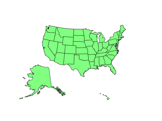
Read a shapefile, containing polygon shapes for each of the US states and the District of Columbia, into a geospatial table. Find the table rows for the conterminous USA, Alaska, and Hawaii.
states = readgeotable("usastatelo.shp");
rowConus = states.Name ~= "Hawaii" & states.Name ~= "Alaska";
rowAlaska = states.Name == "Alaska";
rowHawaii = states.Name == "Hawaii";
Display each of the three regions on separate axes.
figure
ax = usamap("all");
set(ax,"Visible","off")
stateColor = [0.5 1 0.5];

geoshow(ax(1),states(rowConus,:), "FaceColor",stateColor)
geoshow(ax(2),states(rowAlaska,:),"FaceColor",stateColor)
geoshow(ax(3),states(rowHawaii,:),"FaceColor",stateColor)
Hide the frame.
for k = 1:3
    setm(ax(k),"Frame","off","Grid","off",...
      "ParallelLabel","off","MeridianLabel","off")
end
Input Arguments
Output Arguments
Tips
All axes created with
usamapare initialized with a spherical Earth model having a radius of 6,371,000 meters.In some cases,
usamapusestightmapto adjust the axis limits tight around the map. If you change the projection, or just want more white space around the map frame, usetightmapagain oraxis auto.axes(h(n)), wheren = 1,2, or3, makes the desired axes current.set(h,'Visible','on')makes the axes visible.axesscale(h(1))resizes the axes containing Alaska and Hawaii to the same scale as the conterminous states.