stateEstimatorPF
Create particle filter state estimator
Description
The stateEstimatorPF object is a recursive, Bayesian state estimator
that uses discrete particles to approximate the posterior distribution of the estimated
state.
The particle filter algorithm computes the state estimate recursively and involves two steps: prediction and correction. The prediction step uses the previous state to predict the current state based on a given system model. The correction step uses the current sensor measurement to correct the state estimate. The algorithm periodically redistributes, or resamples, the particles in the state space to match the posterior distribution of the estimated state.
The estimated state consists of state variables. Each particle represents a discrete state hypothesis of these state variables. The set of all particles is used to help determine the final state estimate.
You can apply the particle filter to arbitrary nonlinear system models. Process and measurement noise can follow arbitrary non-Gaussian distributions.
For more information on the particle filter workflow and setting specific parameters, see:
Creation
Syntax
Description
pf = stateEstimatorPFinitialize method to initialize the
particles with a known mean and covariance or uniformly distributed particles
within defined bounds. To customize the particle filter’s system and measurement
models, modify the StateTransitionFcn and
MeasurementLikelihoodFcn properties.
After you create the object, use initialize to
initialize the NumStateVariables and
NumParticles properties. The initialize
function sets these two properties based on your inputs.
Properties
Object Functions
initialize | Initialize the state of the particle filter |
getStateEstimate | Extract best state estimate and covariance from particles |
predict | Predict state of robot in next time step |
correct | Adjust state estimate based on sensor measurement |
Examples
Create a stateEstimatorPF object, and execute a prediction and correction step for state estimation. The particle filter gives a predicted state estimate based on the return value of StateTransitionFcn. It then corrects the state based on a given measurement and the return value of MeasurementLikelihoodFcn.
Create a particle filter with the default three states.
pf = stateEstimatorPF
pf =
  stateEstimatorPF with properties:

           NumStateVariables: 3
                NumParticles: 1000
          StateTransitionFcn: @nav.algs.gaussianMotion
    MeasurementLikelihoodFcn: @nav.algs.fullStateMeasurement
     IsStateVariableCircular: [0 0 0]
            ResamplingPolicy: [1×1 resamplingPolicyPF]
            ResamplingMethod: 'multinomial'
       StateEstimationMethod: 'mean'
            StateOrientation: 'row'
                   Particles: [1000×3 double]
                     Weights: [1000×1 double]
                       State: 'Use the getStateEstimate function to see the value.'
             StateCovariance: 'Use the getStateEstimate function to see the value.'
Specify the mean state estimation method and systematic resampling method.
pf.StateEstimationMethod = 'mean';
pf.ResamplingMethod = 'systematic';
Initialize the particle filter at state [4 1 9] with unit covariance (eye(3)). Use 5000 particles.
initialize(pf,5000,[4 1 9],eye(3));
Assuming a measurement [4.2 0.9 9], run one predict and one correct step.
[statePredicted,stateCov] = predict(pf);
[stateCorrected,stateCov] = correct(pf,[4.2 0.9 9]);
Get the best state estimate based on the StateEstimationMethod algorithm.
stateEst = getStateEstimate(pf)
stateEst = 1×3

    4.1562    0.9185    9.0202
Use the stateEstimatorPF object to track a robot as it moves in a 2-D space. The measured position has random noise added. Using predict and correct, track the robot based on the measurement and on an assumed motion model.
Initialize the particle filter and specify the default state transition function, the measurement likelihood function, and the resampling policy.
pf = stateEstimatorPF;
pf.StateEstimationMethod = 'mean';
pf.ResamplingMethod = 'systematic';
Sample 1000 particles with an initial position of [0 0] and unit covariance.
initialize(pf,1000,[0 0],eye(2));
Prior to estimation, define a sine wave path for the dot to follow. Create an array to store the predicted and estimated position. Define the amplitude of noise.
t = 0:0.1:4*pi;
dot = [t; sin(t)]';
robotPred = zeros(length(t),2);
robotCorrected = zeros(length(t),2);
noise = 0.1;
Begin the loop for predicting and correcting the estimated position based on measurements. The resampling of particles occurs based on theResamplingPolicy property. The robot moves based on a sine wave function with random noise added to the measurement.
for i = 1:length(t)
    % Predict next position. Resample particles if necessary.
    [robotPred(i,:),robotCov] = predict(pf);
    % Generate dot measurement with random noise. This is
    % equivalent to the observation step.
    measurement(i,:) = dot(i,:) + noise*(rand([1 2])-noise/2);
    % Correct position based on the given measurement to get best estimation.
    % Actual dot position is not used. Store corrected position in data array.
    [robotCorrected(i,:),robotCov] = correct(pf,measurement(i,:));
end
Plot the actual path versus the estimated position. Actual results may vary due to the randomness of particle distributions.
plot(dot(:,1),dot(:,2),robotCorrected(:,1),robotCorrected(:,2),'or')
xlim([0 t(end)])
ylim([-1 1])
legend('Actual position','Estimated position')
grid on
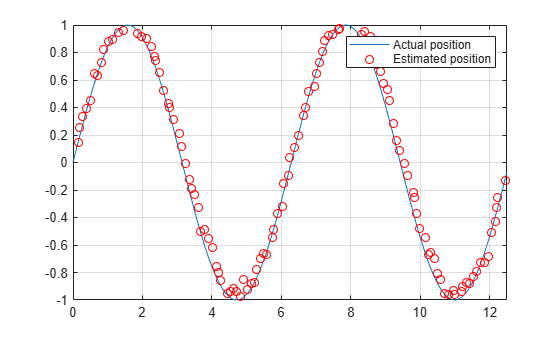
The figure shows how close the estimate state matches the actual position of the robot. Try tuning the number of particles or specifying a different initial position and covariance to see how it affects tracking over time.
References
[1] Arulampalam, M.S., S. Maskell, N. Gordon, and T. Clapp. "A Tutorial on Particle Filters for Online Nonlinear/Non-Gaussian Bayesian Tracking." IEEE Transactions on Signal Processing. Vol. 50, No. 2, Feb 2002, pp. 174-188.
[2] Chen, Z. "Bayesian Filtering: From Kalman Filters to Particle Filters, and Beyond." Statistics. Vol. 182, No. 1, 2003, pp. 1-69.
Extended Capabilities
Version History
Introduced in R2016aSee Also
resamplingPolicyPF | initialize | getStateEstimate | predict | correct
Topics
- Track a Car-Like Robot Using Particle Filter (Robotics System Toolbox)
- Particle Filter Parameters
- Particle Filter Workflow