Monte Carlo Localization Algorithm
Overview
The Monte Carlo Localization (MCL) algorithm is used to estimate the position and orientation
of a robot. The algorithm uses a known map of the environment, range sensor data, and
odometry sensor data. To see how to construct an object and use this algorithm, see
monteCarloLocalization.
To localize the robot, the MCL algorithm uses a particle filter to estimate its position. The particles represent the distribution of the likely states for the robot. Each particle represents a possible robot state. The particles converge around a single location as the robot moves in the environment and senses different parts of the environment using a range sensor. The robot motion is sensed using an odometry sensor.
The particles are updated in this process:
Particles are propagated based on the change in the pose and the specified motion model,
MotionModel.The particles are assigned weights based on the likelihood of receiving the range sensor reading for each particle. This reading is based on the sensor model you specify in
SensorModel.Based on these weights, a robot state estimate is extracted based on the particle weights. The group of particles with the highest weight is used to estimate the position of the robot.
Finally, the particles are resampled based on the specified
ResamplingInterval. Resampling adjusts particle positions and improves performance by adjusting the number of particles used. It is a key feature for adjusting to changes and keeping particles relevant for estimating the robot state.
The algorithm outputs the estimated pose and covariance. These estimates are the mean and covariance of the highest weighted cluster of particles. For continuous tracking, repeat these steps in a loop to propagate particles, evaluate their likelihood, and get the best state estimate.
For more information on particle filters as a general application, see Particle Filter Workflow.
State Representation
When working with a localization algorithm, the goal is to estimate the state of your system.
For robotics applications, this estimated state is usually a robot pose. For the
monteCarloLocalization object, you specify this pose as a
three-element vector. The pose corresponds to an x-y position,
[x y], and an angular orientation,
theta.

The MCL algorithm estimates these three values based on sensor inputs of the environment and a
given motion model of your system. The output from using the
monteCarloLocalization object includes the
pose, which is the best estimated state of the [x y
theta] values. Particles are distributed around an initial pose,
InitialPose, or sampled uniformly using global localization. The
pose is computed as the mean of the highest weighted cluster of particles once these
particles have been corrected based on measurements.
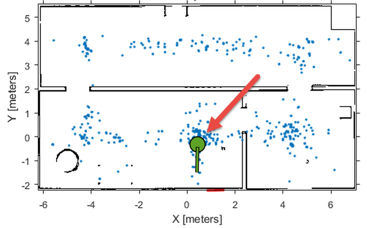
This plot shows the highest weighted cluster and the final robot pose displayed over the
samples particles in green. With more iterations of the MCL algorithm and measurement
corrections, the particles converge to the true location of the robot. However, it is
possible that particle clusters can have high weights for false estimates and converge
on the wrong location. If the wrong convergence occurs, resample the particles by
resetting the MCL algorithm with an updated InitialPose.
Initialization of Particles
When you first create the monteCarloLocalization algorithm, specify the
minimum and maximum particle limits by using the ParticleLimits
property. A higher number of particles increases the likelihood that the particles
converge on the actual location. However, a lower particle number is faster. The number
of particles adjusts dynamically within the limits based on the weights of particle
clusters. This adjustment helps to reduce the number of particles over time so
localization can run more efficiently.
Particle Distribution
Particles must be sampled across a specified distribution. To
initialize particles in the state space, you can use either an initial
pose or global localization. With global localization, you can uniformly
distribute particles across your expected state space (pulled from
the Map property of yourSensorModel object).
In the default MCL object, set the GlobalLocalization property
to true.
mcl = monteCarloLocalization;
mcl.GlobalLocalization = true;

Global localization requires a larger number of particles to effectively sample particles across the state space. More particles increase the likelihood of successful convergence on the actual state. This large distribution greatly reduces initial performance until particles begin to converge and particle number can be reduced.
By default, global localization is set to false. Without global
localization, you must specify the InitialPose and
InitialCovariance properties, which helps to localize the
particles. Using this initial pose, particles are more closely grouped around an
estimated state. A close grouping of particles enables you to use fewer of them, and
increases the speed and accuracy of tracking during the first iterations.

These images were taken from the Localize TurtleBot Using Monte Carlo Localization Algorithm example, which shows how to use the MCL algorithm with the TurtleBot® in a known environment.
Resampling Particles and Updating Pose
To localize your robot continuously, you must resample the particles and update the algorithm.
Use the UpdateThreshold and ResamplingInterval
properties to control when resampling and updates to the estimated state occur.
The UpdateThreshold is a three-element vector that defines the minimum
change in the robot pose, [x y theta], to trigger an update. Changing
a variable by more than this minimum triggers an update, causing the object to return a
new state estimate. This change in robot pose is based on the odometry, which is
specified in the functional form of the object. Tune these thresholds based on your
sensor properties and the motion of your robot. Random noise or minor variations greater
than your threshold can trigger an unnecessary update and affect your performance. The
ResamplingInterval property defines the number of updates to
trigger particle resampling. For example, a resampling interval of 2
resamples at every other update.
The benefit of resampling particles is that you update the possible locations that contribute to the final estimate. Resampling redistributes the particles based on their weights and evolves particles based on the Motion Model. In this process, the particles with lower weight are eliminated, helping the particles converge to the true state of the robot. The number of particles dynamically changes to improve speed or tracking.
The performance of the algorithm depends on proper resampling.
If particles are widely dispersed and the initial pose of the robot
is not known, the algorithm maintains a high particle count. As the
algorithm converges on the true location, it reduces the number of
particles and increases the speed of performance. You can tune your ParticleLimits property
to limit the minimum and maximum particles used to help with the performance.
Motion and Sensor Model
The motion and sensor models for the MCL algorithm are similar to the
StateTransitionFcn and
MeasurementLikelihoodFcn functions for the stateEstimatorPF object, which are described in Particle Filter Parameters. For the MCL algorithm, these models are more
specific to robot localization. After calling the object, to change the
MotionModel or SensorModel properties, you
must first call release on your object.
Sensor Model
By default, the monteCarloLocalization uses a likelihoodFieldSensorModel object as the sensor model. This sensor
model contains parameters specific to the range sensor used, 2-D map information for
the robot environment, and measurement noise characteristics. The sensor model uses
the parameters with range measurements to compute the likelihood of the measurements
given the current position of the robot. Without factoring in these parameters, some
measurement errors can skew the state estimate or increase weight on irrelevant
particles.
The range sensor properties are:
SensorPose– The pose of the range sensor relative to the robot location. This pose is used to transform the range readings into the robot coordinate frame.SensorLimits– The minimum and maximum range limits. Measurement outside of these ranges are not factored into the likelihood calculation.NumBeams– Number of beams used to calculate likelihood. You can improve performance speed by reducing the number of beams used.
Range measurements are also known to give false readings due to system noise or other environmental interference. To account for the sensor error, specify these parameters:
MeasurementNoise– Standard deviation for measurement noise. This deviation applies to the range reading and accounts for any interference with the sensor. Set this value based on information from your range sensor.RandomMeasurementWeight— Weight for probability of random measurement. Set a low probability for random measurements. The default is 0.05.ExpectedMeasurementWeight— Weight for probability of expected measurement. Set a high probability for expected measurements. The default is 0.95.
The sensor model also stores a map of the robot environment as an occupancy grid. Use binaryOccupancyMap to specify your map with occupied and free spaces.
Set any unknown spaces in the map as free locations. Setting them to free locations
prevents the algorithm from matching detected objects to these areas of the
map.

Also, you can specify MaximumLikelihoodDistance,
which limits the area for searching for obstacles. The value of MaximumLikelihoodDistance is
the maximum distance to the nearest obstacle that is used for likelihood
computation.
Motion Model
The motion model for robot localization helps to predict how particles evolve throughout time
when resampling. It is a representation of robot kinematics. The motion model
included by default with the MCL algorithm is an odometry-based differential drive
motion model (odometryMotionModel). Without a motion
model, predicting the next step is more difficult. It is important to know the
capabilities of your system so that the localization algorithm can plan particle
distributions to get better state estimates. Be sure to consider errors from the
wheel encoders or other sensors used to measure the odometry. The errors in the
system define the spread of the particle distribution.
You can specify the error expected based on the motion of your
robot as a four-element vector, Noise. These four
elements are specified as weights on the standard deviations for [1]:
Rotational error due to rotational motion
Rotational error due to translational motion
Translational error due to translational motion
Translational error due to rotational motion
For differential drive robots, when a robot moves from a starting pose to a final pose, the change in pose can be treated as:
Rotation to the final position
Translation in a direct line to the final position
Rotation to the goal orientation
Assuming these steps, you can visualize the effect of errors in rotation and translation. Errors in the initial rotation result in your possible positions being spread out in a C-shape around the final position.
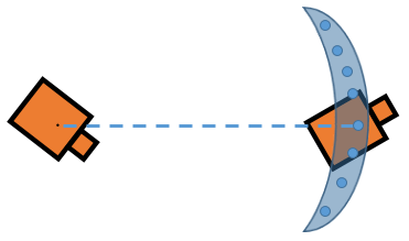
Large translational errors result in your possible positions being spread out around the direct line to the final position.
![]()
Large errors in both translation and rotation can result in wider-spread positions.

Also, rotational errors affect the orientation of the final pose. Understanding these effects
helps you to define the Gaussian noise in the Noise property of
the MotionModel object for your specific application. As the
images show, each parameter does not directly control the dispersion and can vary
with your robot configuration and geometry. Also, multiple pose changes as the robot
navigates through your environment can increase the effects of these errors over
many different steps. By accurately defining these parameters, particles are
distributed appropriately to give the MCL algorithm enough hypotheses to find the
best estimate for the robot location.
References
[1] Thrun, Sebastian, and Dieter Fox. Probabilistic Robotics. 3rd ed. Cambridge, Mass: MIT Press, 2006. p.136.
See Also
monteCarloLocalization | likelihoodFieldSensorModel | odometryMotionModel