gradient
(Not recommended) Evaluate gradient of function approximator object given observation and action input data
Since R2022a
gradient is not recommended. Use the dlgradient and
dlfeval functions
on your loss function instead. For more information, see gradient is not recommended.
Syntax
Description
Examples
Create observation and action specification objects (or
alternatively use the getObservationInfo and
getActionInfo functions to extract the specification objects from
an environment). For this example, define an observation space with three channels. The
first channel carries an observation from a continuous three-dimensional space, so that
a single observation is a column vector containing three doubles. The second channel
carries a discrete observation made of a two-dimensional row vector that can take one of
five different values. The third channel carries a discrete scalar observation that can
be either zero or one. Finally, the action space is a continuous four-dimensional space,
so that a single action is a column vector containing four doubles, each between
-10 and 10.
obsInfo = [
    rlNumericSpec([3 1])
    rlFiniteSetSpec({[1 2],[3 4],[5 6],[7 8],[9 10]})
    rlFiniteSetSpec([0 1])
    ];

actInfo = rlNumericSpec([4 1], ...
                UpperLimit= 10*ones(4,1), ...
                LowerLimit=-10*ones(4,1) );
To approximate the policy within the actor, use a recurrent deep neural network. For a continuous Gaussian actor, the network must have two output layers (one for the mean values the other for the standard deviation values), each having as many elements as the dimension of the action space.
Create a the network, defining each path as an array of layer objects. Use
sequenceInputLayer as the input layer and include an
lstmLayer as one of the other network layers. Also use a softplus
layer to enforce nonnegativity of the standard deviations and a ReLU layer to scale the
mean values to the desired output range. Get the dimensions of the observation and
action spaces from the environment specification objects, and specify a name for the
input layers, so you can later explicitly associate them with the appropriate
environment channel.
obs1Path = [
    sequenceInputLayer( ...
        prod(obsInfo(1).Dimension), ...
        Name="obs1InLyr")
    fullyConnectedLayer(32,Name="obs1PthOutLyr")
    ];

obs2Path = [
    sequenceInputLayer( ...
        prod(obsInfo(2).Dimension), ...
        Name="obs2InLyr")
    fullyConnectedLayer(32,Name="obs2PthOutLyr")
    ];

obs3Path = [
    sequenceInputLayer( ...
        prod(obsInfo(3).Dimension), ...
        Name="obs3InLyr")
    fullyConnectedLayer(32,Name="obs3PthOutLyr")
    ];

% Concatenate inputs along the first available dimension
comPath = [
    concatenationLayer(1,3,Name="comPthInLyr")
    reluLayer
    lstmLayer(8,OutputMode="sequence",Name="lstm")
    fullyConnectedLayer(16)
    reluLayer(Name="comPthOutLyr")
    ];

% Path layers for mean value
% Using tanhLayer & scalingLayer to scale range from (-1,1) to (-10,10)
meanPath = [
    fullyConnectedLayer(prod(actInfo(1).Dimension), ...
    Name="meanPthInLyr")
    tanhLayer
    scalingLayer(Name="meanOutLyr", ...
        Scale=actInfo(1).UpperLimit)
    ];

% Path layers for standard deviations
% Using softplus layer to make them nonnegative
stdPath = [
    fullyConnectedLayer(prod(actInfo(1).Dimension), ...
    Name="stdPthInLyr")
    softplusLayer(Name="stdOutLyr")
    ];

% Assemble dlnetwork object.
net = dlnetwork;
net = addLayers(net,obs1Path);
net = addLayers(net,obs2Path);
net = addLayers(net,obs3Path);
net = addLayers(net,comPath);
net = addLayers(net,meanPath);
net = addLayers(net,stdPath);

% Connect layers.
net = connectLayers(net,"obs1PthOutLyr","comPthInLyr/in1");
net = connectLayers(net,"obs2PthOutLyr","comPthInLyr/in2");
net = connectLayers(net,"obs3PthOutLyr","comPthInLyr/in3");
net = connectLayers(net,"comPthOutLyr","meanPthInLyr/in");
net = connectLayers(net,"comPthOutLyr","stdPthInLyr/in");

% Plot network.
plot(net)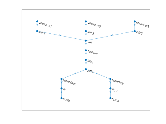
% Initialize network.
net = initialize(net);

% Display the number of learnable parameters.
summary(net)
   Initialized: true

   Number of learnables: 3.9k

   Inputs:
      1   'obs1InLyr'   Sequence input with 3 dimensions
      2   'obs2InLyr'   Sequence input with 2 dimensions
      3   'obs3InLyr'   Sequence input with 1 dimensions
Create the actor with rlContinuousGaussianActor, using the network,
the observations and action specification objects, as well as the names of the network
input layer and the options object.
actor = rlContinuousGaussianActor(net, obsInfo, actInfo, ...
    ActionMeanOutputNames="meanOutLyr", ...
    ActionStandardDeviationOutputNames="stdOutLyr", ...
    ObservationInputNames=["obs1InLyr","obs2InLyr","obs3InLyr"]);
To return mean value and standard deviations of the Gaussian distribution as a
function of the current observation, use the evaluate
function.
[prob,state] = evaluate(actor, {rand([obsInfo(1).Dimension 1 1]) , ...
                                rand([obsInfo(2).Dimension 1 1]) , ...
                                rand([obsInfo(3).Dimension 1 1]) });
The result is a cell array with two elements, the first one containing a vector of mean values, and the second containing a vector of standard deviations.
prob{1}ans = 4×1 single column vector
0.0408
0.1472
-0.0644
-0.0433
prob{2}ans = 4×1 single column vector
0.6966
0.6921
0.6795
0.6859
To return an action sampled from the distribution, use the
getAction function.
act = getAction(actor, {rand(obsInfo(1).Dimension) , ...
                        rand(obsInfo(2).Dimension) , ...
                        rand(obsInfo(3).Dimension) });
act{1}
ans = 4×1 single column vector
-0.0170
1.8817
0.4884
-0.4666
Calculate the gradients of the sum of the outputs (all the mean values plus all the standard deviations) with respect to the inputs, given a random observation.
gro = gradient(actor,"output-input", ...
                        {rand(obsInfo(1).Dimension) , ...
                         rand(obsInfo(2).Dimension) , ...
                         rand(obsInfo(3).Dimension)} )
gro=3×1 cell array
    {3×1 single      }
    {[-0.0424 0.0307]}
    {[        0.0499]}
The result is a cell array with as many elements as the number of input channels. Each element contains the derivatives of the sum of the outputs with respect to each component of the input channel. Display the gradient with respect to the element of the second channel.
gro{2}ans = 1×2 single row vector
-0.0424 0.0307
Obtain the gradient with respect of five independent sequences, each one made of nine sequential observations.
gro_batch = gradient(actor,"output-input", ...
                        {rand([obsInfo(1).Dimension 5 9]) , ...
                         rand([obsInfo(2).Dimension 5 9]) , ...
                         rand([obsInfo(3).Dimension 5 9])} )
gro_batch=3×1 cell array
    {3×1×5×9 single}
    {1×2×5×9 single}
    {1×1×5×9 single}
Display the derivative of the sum of the outputs with respect to the third observation element of the first input channel, after the seventh sequential observation in the fourth independent batch.
gro_batch{1}(3,1,4,7)ans = single
-0.2679
Set the option to accelerate the gradient computations.
actor = accelerate(actor,true);
Calculate the gradients of the sum of the outputs with respect to the parameters, given a random observation.
grp = gradient(actor,"output-parameters", ...
                {rand(obsInfo(1).Dimension) , ...
                 rand(obsInfo(2).Dimension) , ...
                 rand(obsInfo(3).Dimension)} )
grp=15×1 cell array
    {32×3  single}
    {32×1  single}
    {32×2  single}
    {32×1  single}
    {32×1  single}
    {32×1  single}
    {32×96 single}
    {32×8  single}
    {32×1  single}
    {16×8  single}
    {16×1  single}
    { 4×16 single}
    { 4×1  single}
    { 4×16 single}
    { 4×1  single}
Each array within a cell contains the gradient of the sum of the outputs with respect to a group of parameters.
grp_batch = gradient(actor,"output-parameters", ...
                        {rand([obsInfo(1).Dimension 5 9]) , ...
                         rand([obsInfo(2).Dimension 5 9]) , ...
                         rand([obsInfo(3).Dimension 5 9])} )
grp_batch=15×1 cell array
    {32×3  single}
    {32×1  single}
    {32×2  single}
    {32×1  single}
    {32×1  single}
    {32×1  single}
    {32×96 single}
    {32×8  single}
    {32×1  single}
    {16×8  single}
    {16×1  single}
    { 4×16 single}
    { 4×1  single}
    { 4×16 single}
    { 4×1  single}
If you use a batch of inputs, gradient uses the whole input
sequence (in this case nine steps), and all the gradients with respect to the
independent batch dimensions (in this case five) are added together. Therefore, the
returned gradient has always the same size as the output from getLearnableParameters.
Create observation and action specification objects (or
alternatively use the getObservationInfo and
getActionInfo functions to extract the specification objects from
an environment). For this example, define an observation space made of two channels. The
first channel carries an observation from a continuous four-dimensional space. The
second carries a discrete scalar observation that can be either zero or one. Finally,
the action space consists of a scalar that can be -1,
0, or 1.
obsInfo = [
rlNumericSpec([4 1])
rlFiniteSetSpec([0 1])
];
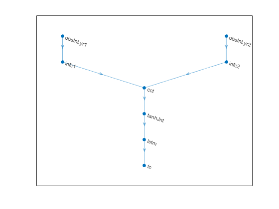
actInfo = rlFiniteSetSpec([-1 0 1]);To approximate the vector Q-value function within the critic, use a recurrent deep neural network. The output layer must have three elements, each one expressing the value of executing the corresponding action, given the observation.
Create the neural network, defining each network path as an array of layer objects.
Get the dimensions of the observation and action spaces from the environment
specification objects, use sequenceInputLayer as the input layer, and
include an lstmLayer as one of the other network layers.
% First path
inPath1 = [
    sequenceInputLayer( ...
        prod(obsInfo(1).Dimension), ...
        Name="obsInLyr1")
    fullyConnectedLayer( ...
        prod(actInfo.Dimension), ...
        Name="infc1")
        ];

% Second path
inPath2 = [
    sequenceInputLayer( ...
         prod(obsInfo(2).Dimension), ...
         Name="obsInLyr2")
    fullyConnectedLayer( ...
         prod(actInfo.Dimension), ...
         Name="infc2")
         ];

% Concatenate inputs along first available dimension.
jointPath = [
    concatenationLayer(1,2,Name="cct")
    tanhLayer(Name="tanhJnt")
    lstmLayer(8,OutputMode="sequence")
    fullyConnectedLayer(prod(numel(actInfo.Elements)))
    ];
Assemble dlnetwork object and add layers.
net = dlnetwork;
net = addLayers(net,inPath1);
net = addLayers(net,inPath2);
net = addLayers(net,jointPath);
Connect layers.
net = connectLayers(net,"infc1","cct/in1");
net = connectLayers(net,"infc2","cct/in2");
Plot network.
plot(net)
Initialize the network.
net = initialize(net);
Display the number of weights.
summary(net)
   Initialized: true

   Number of learnables: 386

   Inputs:
      1   'obsInLyr1'   Sequence input with 4 dimensions
      2   'obsInLyr2'   Sequence input with 1 dimensions
Create the critic with rlVectorQValueFunction, using the network
and the observation and action specification objects.
critic = rlVectorQValueFunction(net,obsInfo,actInfo);
To return the value of the actions as a function of the current observation, use the
getValue or evaluate functions.
val = evaluate(critic, ...
                {rand(obsInfo(1).Dimension), ...
                 rand(obsInfo(2).Dimension)})
val = 1×1 cell array
    {3×1 single}
When you use the evaluate function, the result is a
single-element cell array, containing a vector with the values of all the possible
actions, given the observation.
val{1}ans = 3×1 single column vector
0.1293
-0.0549
0.0425
Calculate the gradients of the sum of the outputs with respect to the inputs, given a random observation.
gro = gradient(critic,"output-input", ...
                {rand(obsInfo(1).Dimension) , ...
                 rand(obsInfo(2).Dimension) } )
gro=2×1 cell array
    {4×1 single}
    {[  0.0611]}
The result is a cell array with as many elements as the number of input channels. Each element contains the derivative of the sum of the outputs with respect to each component of the input channel. Display the gradient with respect to the element of the second channel.
gro{2}ans = single
0.0611
Obtain the gradient with respect of five independent sequences each one made of nine sequential observations.
gro_batch = gradient(critic,"output-input", ...
                        {rand([obsInfo(1).Dimension 5 9]) , ...
                         rand([obsInfo(2).Dimension 5 9]) } )
gro_batch=2×1 cell array
    {4×1×5×9 single}
    {1×1×5×9 single}
Display the derivative of the sum of the outputs with respect to the third observation element of the first input channel, after the seventh sequential observation in the fourth independent batch.
gro_batch{1}(3,1,4,7)ans = single
-0.1192
Set the option to accelerate the gradient computations.
critic = accelerate(critic,true);
Calculate the gradients of the sum of the outputs with respect to the parameters, given a random observation.
grp = gradient(critic,"output-parameters", ...
                {rand(obsInfo(1).Dimension) , ...
                 rand(obsInfo(2).Dimension) } )
grp=9×1 cell array
    {[-0.0178 -0.0052 -0.0588 -0.0114]}
    {[                        -0.0597]}
    {[                         0.0873]}
    {[                         0.0962]}
    {32×2 single                      }
    {32×8 single                      }
    {32×1 single                      }
    { 3×8 single                      }
    { 3×1 single                      }
Each array within a cell contains the gradient of the sum of the outputs with respect to a group of parameters.
grp_batch = gradient(critic,"output-parameters", ...
                        {rand([obsInfo(1).Dimension 5 9]) , ...
                         rand([obsInfo(2).Dimension 5 9]) })
grp_batch=9×1 cell array
    {[-2.4487 -2.3282 -2.4941 -2.5877]}
    {[                        -5.1411]}
    {[                         4.4295]}
    {[                         9.2137]}
    {32×2 single                      }
    {32×8 single                      }
    {32×1 single                      }
    { 3×8 single                      }
    { 3×1 single                      }
If you use a batch of inputs, gradient uses the whole input
sequence (in this case nine steps), and all the gradients with respect to the
independent batch dimensions (in this case five) are added together. Therefore, the
returned gradient always has the same size as the output from getLearnableParameters.
Input Arguments
Output Arguments
Version History
Introduced in R2022aSee Also
Functions
Objects
AcceleratedFunction|rlValueFunction|rlQValueFunction|rlVectorQValueFunction|rlContinuousDeterministicActor|rlDiscreteCategoricalActor|rlContinuousGaussianActor|rlContinuousDeterministicTransitionFunction|rlContinuousGaussianTransitionFunction|rlContinuousDeterministicRewardFunction|rlContinuousGaussianRewardFunction|rlIsDoneFunction