Main Content

falltime

Fall time of negative-going bilevel waveform transitions

Description

example

f = falltime(x) returns a vector f containing the time it takes each transition of the bilevel waveform x to cross from the 90% reference level to the 10% reference level.

Note

Because falltime uses interpolation, f may contain values that do not correspond to sampling instants of the bilevel waveform x.

f = falltime(x,fs) specifies the sample rate in hertz. The sample rate determines the sample instants corresponding to the elements in x.

example

f = falltime(x,t) specifies the sample instants t as a vector with the same number of elements as x.

example

[f,lt,ut,ll,ul] = falltime(___) returns the levels ll and ul corresponding to the lower- and upper-percent reference levels.

example

[f,lt,ut] = falltime(___) returns vectors lt and ut whose elements correspond to the time instants where x crosses the lower- and upper-percent reference levels. You can use this output syntax with any of the previous input syntaxes.

example

[___] = falltime(___,Name=Value) returns the fall times with additional options specified by one or more name-value arguments.

example

falltime(___) plots the signal and darkens the regions of each transition where fall time is computed. The plot marks the lower and upper crossings and the associated reference levels. The plot also displays the state levels and the associated lower- and upper-state boundaries.

Examples

collapse all

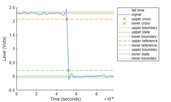
Load data for a 2.3 V clock waveform. Determine the fall time in samples and use the default 10% and 90% reference levels. Plot the waveform and annotate the fall time.

load("negtransitionex")

falltime(x)

Figure Fall Time Plot contains an axes object. The axes object with xlabel Time (seconds), ylabel Level (Volts) contains 12 objects of type patch, line. One or more of the lines displays its values using only markers These objects represent fall time, signal, upper cross, lower cross, upper boundary, upper state, lower boundary, upper reference, lower reference, lower state.

ans = 0.7200

Determine the fall time again and specify the sample instants t. Plot the result in a new figure.

figure
falltime(x,t)

Figure Fall Time Plot contains an axes object. The axes object with xlabel Time (seconds), ylabel Level (Volts) contains 12 objects of type patch, line. One or more of the lines displays its values using only markers These objects represent fall time, signal, upper cross, lower cross, upper boundary, upper state, lower boundary, upper reference, lower reference, lower state.

ans = 1.8000e-07

Determine the fall time in a 2.3 V clock waveform sampled at 4 MHz. Compute the fall time using the 20% and 80% reference levels.

Load the 2.3 V clock data. Determine the fall time using 20% and 80% reference levels and specify a 5% tolerance region. Plot the waveform and annotate the fall time.

load("negtransitionex")

falltime(x,PercentReferenceLevels=[20 80],Tolerance=5)
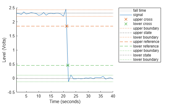
Figure Fall Time Plot contains an axes object. The axes object with xlabel Time (seconds), ylabel Level (Volts) contains 12 objects of type patch, line. One or more of the lines displays its values using only markers These objects represent fall time, signal, upper cross, lower cross, upper boundary, upper state, lower boundary, upper reference, lower reference, lower state.

ans = 0.5400

Determine the fall time, reference level instants, and reference levels in a 2.3 V clock waveform sampled at 4 MHz.

Load the 2.3 V clock waveform data.

load("negtransitionex")

Determine the fall time, reference level instants, and reference levels. Specify the sampling instants t.

[f,lt,ut,ll,ul] = falltime(x,t);

Plot the waveform with the lower- and upper-reference levels and reference level instants. Show that the fall time is the difference between the lower- and upper-reference level instants.

plot(t,x)
xlabel("Seconds")
ylabel("Volts")

hold on
plot([lt ut],[ll ul],"ro")
hold off

Figure contains an axes object. The axes object with xlabel Seconds, ylabel Volts contains 2 objects of type line. One or more of the lines displays its values using only markers

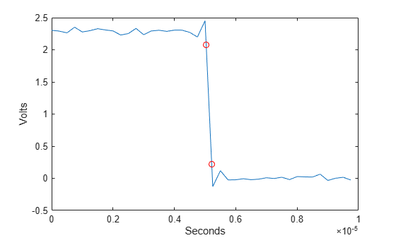
fprintf("Fall time is %g seconds.",lt-ut)
Fall time is 1.8e-07 seconds.

Input Arguments

collapse all

Bilevel waveform, specified as a real-valued vector.

Sample rate, specified as a positive real scalar in hertz. The first sample instant in x corresponds to t = 0.

Sample instants, specified as a vector. The length of t must equal the length of the bilevel waveform x.

Name-Value Arguments

Specify optional pairs of arguments as Name1=Value1,...,NameN=ValueN, where Name is the argument name and Value is the corresponding value. Name-value arguments must appear after other arguments, but the order of the pairs does not matter.

Example: falltime(x,PercentReferenceLevels=[20 80]) computes the fall time using 20% and 80% reference levels.

Before R2021a, use commas to separate each name and value, and enclose Name in quotes.

Example: falltime(x,"PercentReferenceLevels",[20 80])

Reference levels as a percentage of the waveform amplitude, specified as a two-element positive row vector. The elements of the row vector correspond to the lower- and upper-percent reference levels. The high-state level is defined to be 100 percent, and the low-state level is defined to be 0 percent. For more information, see Percent Reference Levels.

Low- and high-state levels, specified as a two-element row vector. The first and second elements of the vector correspond to the low- and high-state levels.

Lower- and upper-state boundaries, specified as a real positive scalar as a percentage value. For more information, see State-Level Tolerances.

Output Arguments

collapse all

Duration of negative-going transition, returned as a vector. If you specify the sample rate fs or the sample instants t, then the fall times are in seconds. If you do not specify a sample rate or sample instants, then the fall times are in samples.

Lower-reference level crossing instants, returned as a vector. The vector lt contains the time instants when the negative-going transition crosses the lower-reference level. By default, the lower-reference level is the 10% reference level. You can change the default reference levels by specifying PercentReferenceLevels.

Upper-reference level crossing instants, returned as a vector. The vector ut contains the time instants when the negative-going transition crosses the upper-reference level. By default, the upper-reference level is the 90% reference level. You can change the default reference levels by specifying PercentReferenceLevels.

Lower-reference level in waveform amplitude units, returned as a real numeric scalar. ll is a vector containing the waveform values corresponding to the lower-reference level in each negative-going transition. By default, the lower-reference level is the 10% reference level. You can change the default reference levels by specifying PercentReferenceLevels.

Upper-reference level in waveform amplitude units, returned as a real numeric scalar. ul is a vector containing the waveform values corresponding to the upper-reference level in each negative-going transition. By default, the upper-reference level is the 90% reference level. You can change the default reference levels by specifying PercentReferenceLevels.

More About

collapse all

Transitions

To determine the transitions, the falltime function estimates the state levels of the input waveform using a histogram method. The function identifies all regions that cross the lower-state boundary of the high state and the upper-state boundary of the low state. The low-state and high-state boundaries are expressed as the state level plus or minus a multiple of the difference between the state levels.

Negative-Going Transition

A negative-going transition in a bilevel waveform is a transition from the high-state level to the low-state level. If the waveform is differentiable in the neighborhood of the transition, an equivalent definition is a transition with a negative first derivative. This figure shows a negative-going transition.

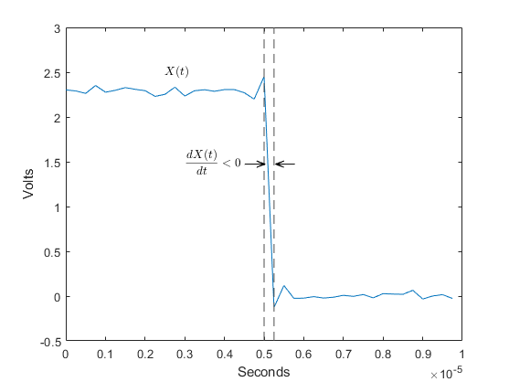
In the preceding figure, the amplitude values of the waveform are not displayed because a negative-going transition does not depend on the actual waveform values. A negative-going transition is defined by the direction of the transition.

Percent Reference Levels

If S1 is the low state, S2 is the high state, and U is the upper-percent reference level. The waveform value corresponding to the upper-percent reference level is

S1+U100(S2S1).

If L is the lower-percent reference level, the waveform value corresponding to the lower-percent reference level is

S1+L100(S2S1).

State-Level Tolerances

You can specify lower- and upper-state boundaries for each state level. Define the boundaries as the state level plus or minus a scalar multiple of the difference between the high state and the low state. To provide a useful tolerance region, specify the scalar as a small number such as 2/100 or 3/100. In general, the $\alpha\%$ region for the low state is defined as

$$S_1\pm{\alpha\over{100}}(S_2-S_1),$$

where $S_1$ is the low-state level and $S_2$ is the high-state level. Replace the first term in the equation with $S_2$ to obtain the $\alpha\%$ tolerance region for the high state.

This figure shows lower and upper 5% state boundaries (tolerance regions) for a positive-polarity bilevel waveform. The thick dashed lines indicate the estimated state levels.

References

[1] IEEE® Standard on Transitions, Pulses, and Related Waveforms, IEEE Standard 181, 2003, pp. 15–17.

Extended Capabilities

C/C++ Code Generation
Generate C and C++ code using MATLAB® Coder™.

Version History

Introduced in R2012a