risetime
Rise time of positive-going bilevel waveform transitions
Syntax
Description
r = risetime(x)r, containing the time each transition of
the input bilevel waveform, x, takes to cross from the 10%
to 90% reference levels. To determine the transitions,
risetime estimates the state levels of the input
waveform by a histogram method. risetime identifies all
regions that cross the upper-state boundary of the low state and the lower-state
boundary of the high state. The low-state and high-state boundaries are
expressed as the state level plus or minus a multiple of the difference between
the state levels. See State-Level Tolerances. Because risetime
uses interpolation, r can contain values that do not
correspond to sampling instants of the bilevel waveform,
x.
r = risetime(x,fs)x. The first
sample instant in x corresponds to t = 0. Because risetime uses interpolation,
r can contain values that do not correspond to sampling
instants of the bilevel waveform, x.
[___] = risetime(___,
returns the rise times with additional options specified by one or more
name-value arguments.Name=Value)
risetime(___) plots the signal and darkens
the regions of each transition where rise time is computed. The plot marks the
lower and upper crossings and the associated reference levels. The state levels
and the corresponding associated lower- and upper-state boundaries are also
plotted.
Examples
Determine the rise time in samples for a 2.3 V clock waveform.
Load the 2.3 V clock data. Determine the rise time in samples. Use the default 10% and 90% percent reference levels.
load("transitionex.mat","x","t")
R = risetime(x)
R =
0.7120
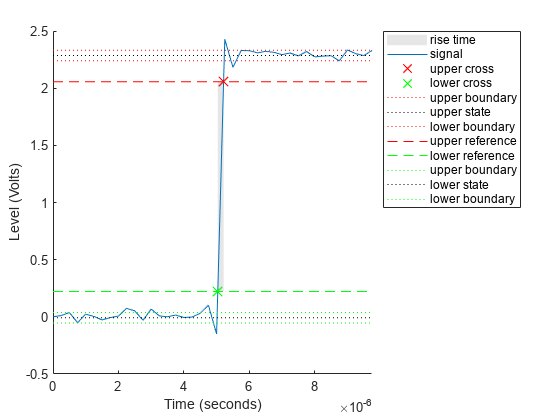
The rise time is less than 1, indicating that the transition occurred in a fraction of a sample. Plot the data, including the time information, and annotate the rise time.
risetime(x,t);
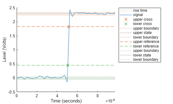
Determine the rise time, reference-level instants, and reference levels in a 2.3 V clock waveform sampled at 4 MHz.
Load the 2.3 V clock waveform along with the sampling instants.
load("transitionex.mat","x","t")
Determine the rise time, reference-level instants, and reference levels.
[R,lt,ut,ll,ul] = risetime(x,t);
Plot the waveform with the lower- and upper-reference levels and reference-level instants. Show that the rise time is the difference between the upper- and lower-reference level instants.
plot(t,x)
xlabel("Seconds")
ylabel("Volts")

hold on
plot([lt ut],[ll ul],"o")
hold off

fprintf('Rise time is %g seconds.',ut-lt)Rise time is 1.78e-07 seconds.
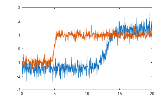
Generate two signals that represent bilevel waveforms. The signals are sampled at 50 Hz for 20 seconds. For the first signal, the transition occurs 13 seconds after the start of the measurement. For the second signal, the transition occurs 5 seconds after the start of the measurement. The signals have different amplitudes and are embedded in white Gaussian noise of different variances. Plot the signals.
tt = linspace(0,20,1001)';
e1 = 1.4*tanh(tt-13)+randn(size(tt))/3;
e2 = tanh(3*(tt-5))+randn(size(tt))/5;

plot(tt,e1,tt,e2)
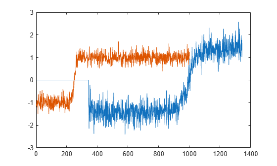
Align the signals so their transition times coincide. Correlation-based methods cannot align this type of signals adequately.
[y1,y2,D] = alignsignals(e1,e2);

plot(y1)
hold on
plot(y2)
hold off
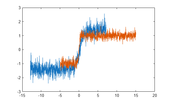
Use risetime to align the signals. For each signal, find the transition time as the average of the instant at which the signal crosses the lower reference level and the instant at which it crosses the upper reference level. Plot the aligned waveforms.
[~,l1,u1] = risetime(e1,tt);
[~,l2,u2] = risetime(e2,tt);

t1 = tt-(l1+u1)/2;
t2 = tt-(l2+u2)/2;

plot(t1,e1,t2,e2)
Determine the rise time in a 2.3 V clock waveform sampled at 4 MHz. Compute the rise time using the 20% and 80% reference levels.
Load the 2.3 V clock data with sampling instants. Compute the sample rate as the inverse of the time difference between consecutive samples. Determine the rise time using the 20% and 80% reference levels. Plot the annotated waveform.
load("transitionex.mat","x","t")

fs = 1/(t(2)-t(1));

risetime(x,fs,PercentReferenceLevels=[20 80])
ans =
1.3350e-07
Input Arguments
Name-Value Arguments
Output Arguments
More About
A positive-going transition in a bilevel waveform is a transition from the low-state level to the high-state level. A positive-polarity (positive-going) pulse has a terminating state more positive than the originating state. If the waveform is differentiable in the neighborhood of the transition, an equivalent definition is a transition with a positive first derivative. This figure shows a positive-going transition.
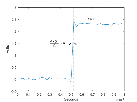
The amplitude values of the waveform do not appear because a positive-going transition does not depend on the actual waveform values. A positive-going transition is defined by the direction of the transition.
You can specify lower- and upper-state boundaries for each state level. Define the boundaries as the state level plus or minus a scalar multiple of the difference between the high state and the low state. To provide a useful tolerance region, specify the scalar as a small number such as 2/100 or 3/100. In general, the region for the low state is defined as
where is the low-state level and is the high-state level. Replace the first term in the equation with to obtain the tolerance region for the high state.
This figure shows lower and upper 5% state boundaries (tolerance regions) for a positive-polarity bi-level waveform. The thick dashed lines indicate the estimated state levels.

References
[1] IEEE® Standard on Transitions, Pulses, and Related Waveforms, IEEE Standard 181, 2003, pp. 15–17.
Extended Capabilities
Version History
Introduced in R2012a