Signal Analyzer

R2026b

Visualize and compare multiple signals and spectra

Description

The Signal Analyzer app is an interactive tool for visualizing, preprocessing, measuring, analyzing, and comparing signals in the time domain, in the frequency domain, and in the time-frequency domain. Using the app, you can:

• Easily access all the signals in the MATLAB^® workspace.

• Fill missing data (since R2024a); smooth, filter, resample, detrend, denoise, extract, and edit signals without leaving the app.

• Add and apply custom preprocessing functions.

• Play audio signals. (since R2024a)

• Visualize and compare multiple waveform, spectrum, persistence, spectrogram, and scalogram representations of signals simultaneously.

• Measure data and signal statistics.

• Work with many signals of varying durations at the same time and in the same view.

For more information, see Use Signal Analyzer App.

Required Products

You need a Wavelet Toolbox™ license to use the scalogram view and to apply wavelet denoising to signals.

Open the Signal Analyzer App

• MATLAB Toolstrip: On the Apps tab, under Signal Processing and Audio, click the app icon.

• MATLAB command prompt: Enter signalAnalyzer.

Examples

Find and Fill Missing Data in Audio File

Load a speech signal sampled at $$F_s=7418Hz$$. The file contains a recording of a female voice saying the word "MATLAB®."

load mtlb

To simulate a situation where 70% of the audio data is missing, randomly assign NaN values to the signal.

rng(2024) 
numToReplace = round(length(mtlb) * 0.70);
missing = randperm(length(mtlb),numToReplace);

mtlbMissing = mtlb;
mtlbMissing(missing) = NaN;

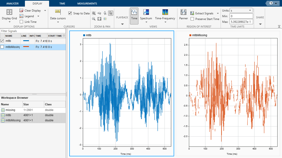
Open Signal Analyzer and drag the mtlb and mtlbMissing variables from the Workspace Browser pane to the Filter Signals table. Press Shift and click each signal name to simultaneously select the two signals. On the Analyzer tab, click Time Values and select Sample Rate and Start Time. Specify Sample Rate as Fs Hz and Start Time as 0 s. Click Display Grid to create two side-by-side displays. Plot mtlb in the left display and mtlbMissing in the right display. To hear the mtlb audio signal, select it and click Play in the Playback section of the toolstrip under the Display tab. To repeat the signal, select Play in Loop before playing.

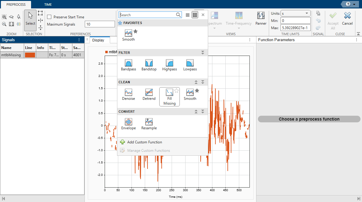
Select the signal with missing data and click Preprocess under the Analyzer tab to enter the preprocessing mode, then select Fill Missing from the gallery of preprocessing functions. Use the Function Parameters panel to adjust the Fill Missing parameters. Set Fill Function to Autoregressive model and click Apply to fill in the missing signal. Click Accept All to save the preprocessing results and exit the mode. For details on alternative fill functions, see fillmissing and fillgaps.

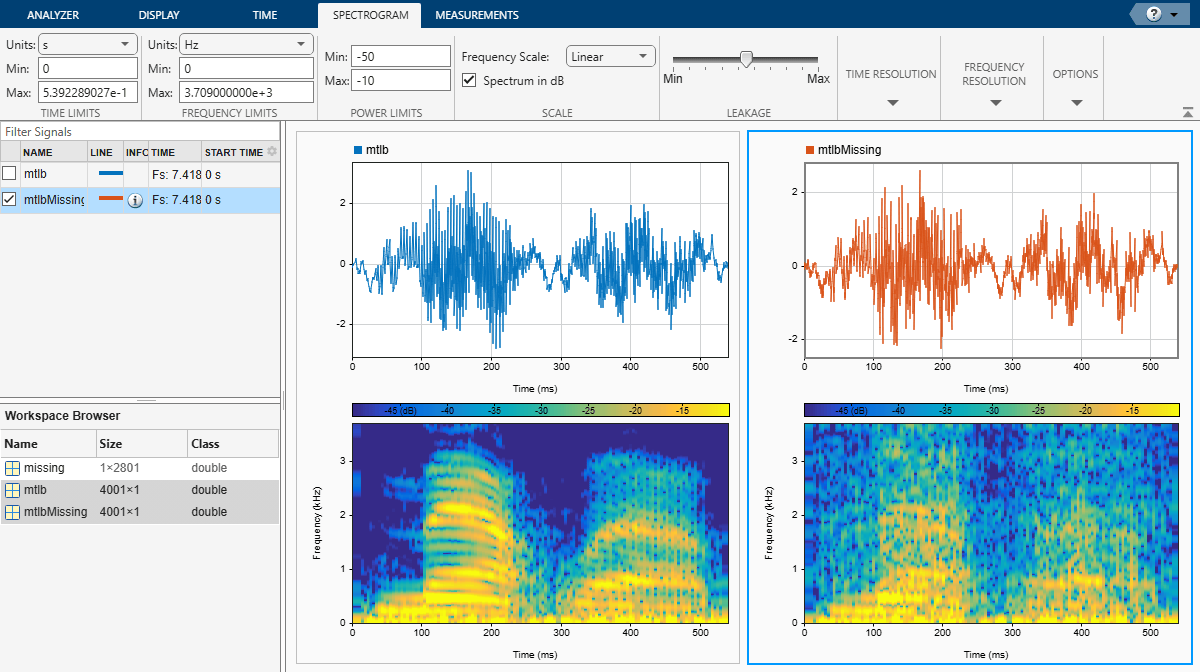
You can now play the filled signal using the Play button. To see the effect of filling missing data on the spectrogram, click Time-Frequency/Spectrogram on the Views section of the Display tab. On the Spectrogram tab, specify a time resolution of 20 ms and 80% overlap between adjoining segments. Set the Power Limits to –50 dB and –10 dB. Click the left display and repeat the steps.

Resolve Tones by Varying Window Leakage

You can adjust the spectral leakage of the analysis window to resolve sinusoids in Signal Analyzer.

Generate a two-channel signal sampled at 100 Hz for 2 seconds.

1. The first channel consists of a 20 Hz tone and a 21 Hz tone. Both tones have unit amplitude.

2. The second channel also has two tones. One tone has unit amplitude and a frequency of 20 Hz. The other tone has an amplitude of 1/100 and a frequency of 30 Hz.

Fs = 100;
t = (0:1/Fs:2-1/Fs)';

x = sin(2*pi*[20 20].*t) + [1 1/100].*sin(2*pi*[21 30].*t);

Embed the signal in white noise. Specify a signal-to-noise ratio of 40 dB.

x = x + randn(size(x)).*std(x)/db2mag(40);

Open Signal Analyzer and plot the signal. On the Analyzer tab, with the signal selected in the Signal table, click Time Values and select Sample Rate and Start Time. Specify Sample Rate as Fs Hz and Start Time as 0 s. On the Display tab, click Spectrum to add a spectral plot to the display.

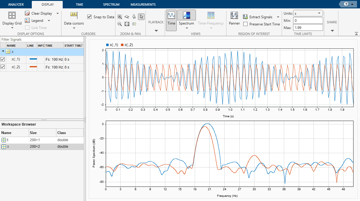
Click the Spectrum tab. The slider that controls the spectral leakage is in the middle position, corresponding to a resolution bandwidth of about 1.28 Hz. The two tones in the first channel are not resolved. The 30 Hz tone in the second channel is visible, despite being much weaker than the other one.

Increase the leakage so that the resolution bandwidth is approximately 0.83 Hz. The weak tone in the second channel is clearly resolved.

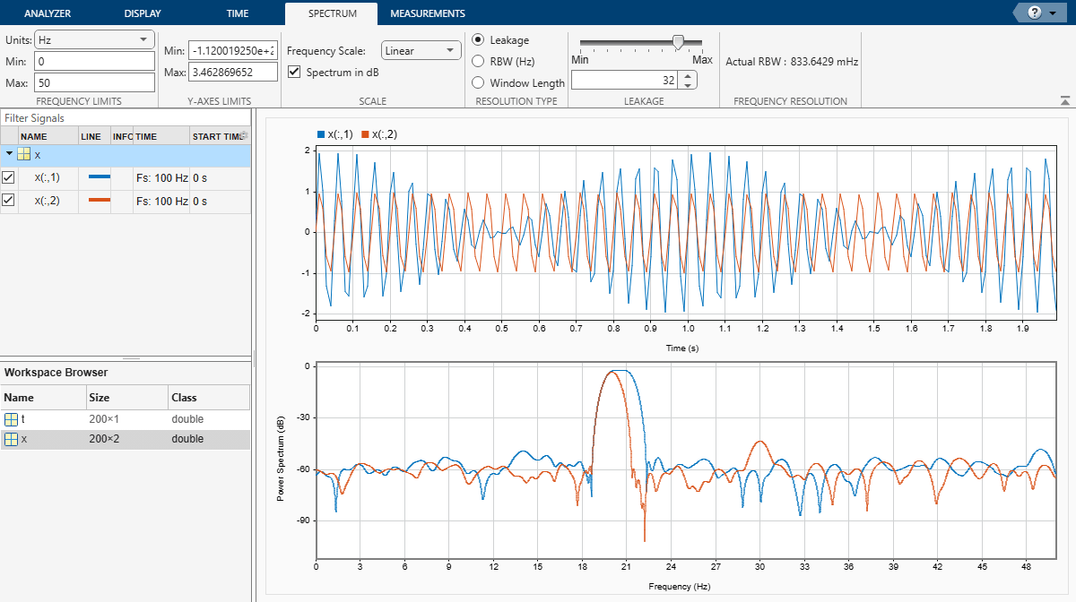
Move the slider to the maximum value. The resolution bandwidth is approximately 0.5 Hz. The two tones in the first channel are resolved. The weak tone in the second channel is masked by the large window sidelobes.

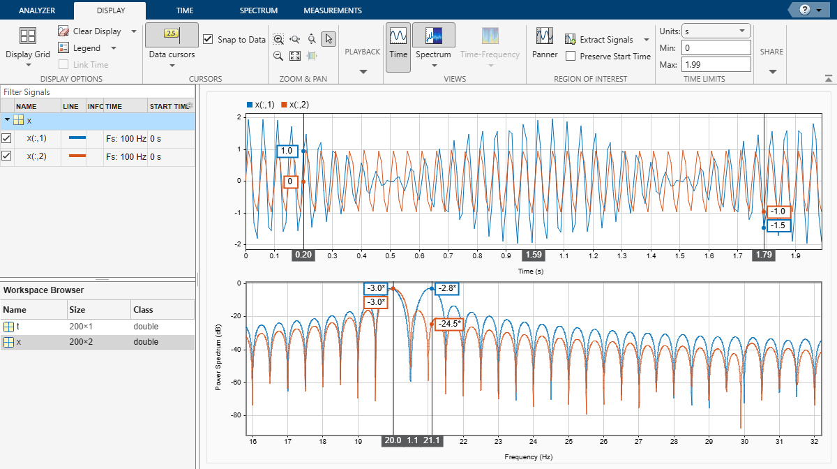
Click the Display tab. Use the horizontal zoom (Zoom in X) to magnify the frequency axis. Add two cursors to the display and drag the frequency-domain cursors to estimate the frequencies of the tones.

Compute Signal Spectrum Using Different Windows

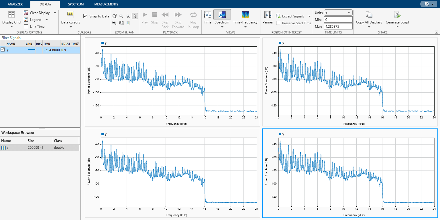
Read an audio recording of an electronic toothbrush into MATLAB®. The signal is sampled at 48 kHz. The toothbrush turns on at about 1.75 seconds and stays on for approximately 2 seconds.

[y,Fs] = audioread("toothbrush.m4a");

Open Signal Analyzer and drag the signal from the Workspace Browser to the Signal table. Add time information to the signal by selecting it in the Signal table and clicking Time Values on the Analyzer tab. Select Sample Rate and Start Time and enter fs for the sample rate.

On the Display tab, click Display Grid to create a two-by-two grid of displays. Select each display, click Spectrum to add a spectrum view, and click Time to remove the time view. Drag the signal to all four displays.

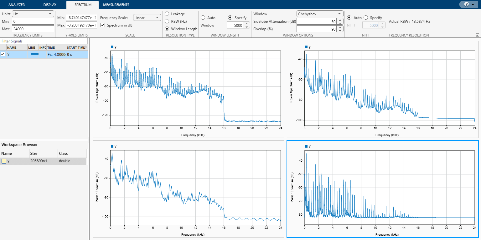
Click the Spectrum tab to modify the spectrum view in each display.

1. Click the top left display to select it. Move the Leakage slider until you get a leakage value of 32.

2. Click the top right display to select it. On the Resolution Type section, select Window Length. On the Window Length section, select Specify and specify a window length of 1500 samples. On the Window Options section, choose a Rectangular window and specify an overlap percentage of 20.

3. Click the bottom left display to select it. On the Resolution Type section, select Window Length. On the Window Length section, select Specify and specify a window length of 500 samples. On the Window Options section, choose a Hamming window and specify an overlap percentage of 50. On the NFFT section, specify 550 discrete Fourier transform points.

4. Click the bottom right display to select it. On the Resolution Type section, select Window Length. On the Window Length section, select Specify and specify a window length of 5000 samples. On the Window Options section, choose a Chebyshev window and specify a sidelobe attenuation of 50 dB and an overlap percentage of 90.

You can see that some views show higher resolution but higher leakage, while other views have lower leakage but at the expense of resolution.

Plot Power Spectrum of Signals with Different Sample Rates

Since R2026b

Use Signal Analyzer to generate a script that plots the power spectrum of signals having different sample rates. Edit the generated script to resample the signals and plot the power spectrum at a common sample rate.

Generate a family of three signals that comprise a sinusoid and a linearly swept chirp. Use different sample rates and amplitudes.

fam = @(a,t) a(1)*sin(2*pi*2*t') + a(2)*chirp(t',4,4,10);
xt1 = timetable(fam([3.5 8.4],0:1/200:10),SampleRate=200);
xt2 = timetable(fam([4.2 6.5],0:1/500:10),SampleRate=500);
xt3 = timetable(fam([3.2 9.3],0:1/1e3:10),SampleRate=1e3);

Open Signal Analyzer and plot the signals in the time domain. To perform this action programmatically, uncomment this command.

% signalAnalyzer(xt1,xt2,xt3)

To plot the power spectrum, select Spectrum in the View section of the Display toolstrip tab. Signal Analyzer plots the power spectrum in a separate display and uses the maximum sample rate between all signals being plotted.

To modify the spectrum view, navigate to the Spectrum toolstrip tab and adjust these settings:

• In the Frequency Limits section, set a maximum frequency of 20 Hz.

• In the Scale section, clear the Spectrum in dB check box.

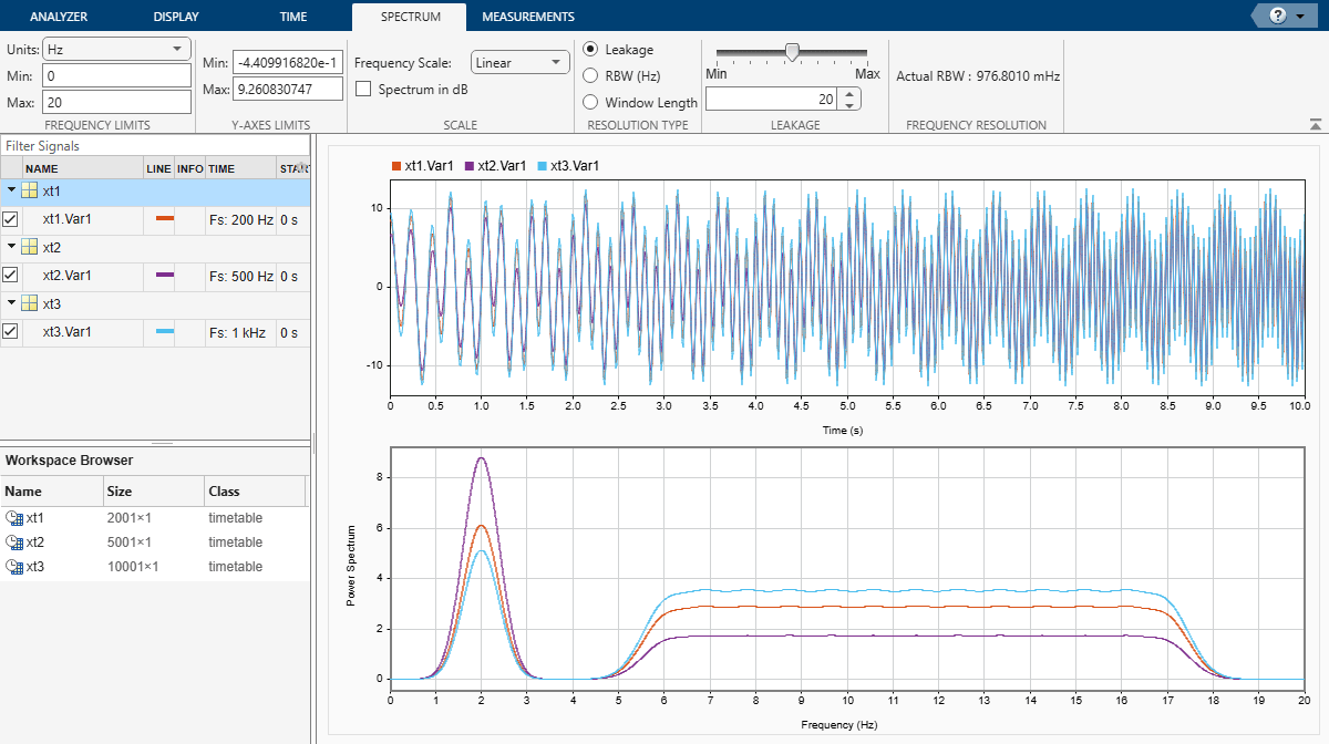
Generate a script that plots the power spectrum of these signals. In the Share section of the Display toolstrip tab, select Generate Script and then Spectrum Script. This example saves the generated script as signalAnalyzerGeneratedScript.m.

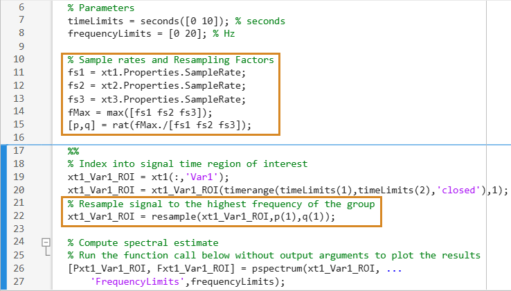
To plot the power spectrum outside of Signal Analyzer when the signals have different sample rates, edit the script generated with Signal Analyzer. Add these code blocks and save the edited script.

Edit Type	Code to Add
Identify sample rates and resampling factors	fs1 = xt1.Properties.SampleRate; fs2 = xt2.Properties.SampleRate; fs3 = xt3.Properties.SampleRate; fMax = max([fs1 fs2 fs3]); [p,q] = rat(fMax./[fs1 fs2 fs3]);
Resample signal 1 to the highest frequency of the group	xt1_Var1_ROI = resample(xt1_Var1_ROI,p(1),q(1));
Resample signal 2 to the highest frequency of the group	xt2_Var1_ROI = resample(xt2_Var1_ROI,p(2),q(2));
Resample signal 3 to the highest frequency of the group	xt3_Var1_ROI = resample(xt3_Var1_ROI,p(3),q(3));

The figure shows where to add the code blocks in the Signal Analyzer script. This example saves the edited script as signalAnalyzerGeneratedScriptEdited.m.

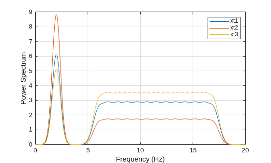
Run the edited script. Plot the power spectrum of the signals. The figure agrees with the power spectrum display in Signal Analyzer.

run("signalAnalyzerGeneratedScriptEdited.m")
plot([Fxt1_Var1_ROI Fxt2_Var1_ROI Fxt3_Var1_ROI], ...
    [Pxt1_Var1_ROI Pxt2_Var1_ROI Pxt3_Var1_ROI])
grid on
legend(["xt1" "xt2" "xt3"])
xlabel("Frequency (Hz)")
ylabel("Power Spectrum")

Related Examples

• Extract Voices from Music Signal
• Modulation and Demodulation Using Complex Envelope
• Find and Track Ridges Using Reassigned Spectrogram
• Declip Saturated Signals Using Your Own Function
• Compute Envelope Spectrum of Vibration Signal
• Find Delay Between Correlated Signals
• Find Interference Using Persistence Spectrum
• Denoise Noisy Doppler Signal
• Resample and Filter a Nonuniformly Sampled Signal
• Extract Regions of Interest from Whale Song

Programmatic Use

signalAnalyzer opens the Signal Analyzer app.

signalAnalyzer(sig) opens the Signal Analyzer app and imports and plots the signal sig. If the app is already open, then it plots sig in the current display. If sig is already plotted but has changed, then the function call updates the plot.

sig can be a variable in the workspace or a MATLAB expression. sig can be:

• A vector or a matrix with independent signals in each column.

• A timetable with time values specified as durations.

• A timeseries object.

See Data Types Supported by Signal Analyzer for more details.

By default, the app plots the signal as a function of sample index. If you provide time information, or if the signal has inherent time information, then the app plots the signal as a function of time.

signalAnalyzer(sig1,...,sigN) imports N signal vectors or matrices and plots them in the current display. The app does not support importing signals with inherent time information and signals without inherent time information in the same function call.

signalAnalyzer(___,SampleRate=fs) specifies a sample rate, fs, as a positive scalar expressed in Hz. The app uses the sample rate to plot one or more signals against time, assuming a start time of zero. You can specify a sample rate for signals with no inherent time information.

signalAnalyzer(___,SampleTime=ts) specifies a sample time, ts, as a positive scalar expressed in seconds. The app uses the sample time to plot one or more signals against time, assuming a start time of zero. You can specify a sample time for signals with no inherent time information.

signalAnalyzer(___,StartTime=st) specifies a signal start time, st, as a scalar expressed in seconds. If you do not specify a sample rate or sample time, then the app assumes a sample rate of 1 Hz. You can specify a start time for signals with no inherent time information.

signalAnalyzer(___,TimeValues=tv) specifies a vector, tv, with time values corresponding to the data points. tv can be a real numeric vector with values expressed in seconds. tv can also be a duration array. The values in tv must be unique and cannot be NaN, but they need not be uniformly spaced. All input signals must have the same length as tv. You can specify a vector of time values for signals with no inherent time information.

Filtering and scalogram view do not support nonuniformly sampled signals.

Version History

Introduced in R2016a

R2024a: Find and fill missing data

Preprocess signals in the Signal Analyzer app by finding and filling gaps in the data. You can fill missing data with constant values, combinations of neighboring samples, or moving averages. You can also interpolate or apply an autoregressive model.

R2024a: Play audio signals

Play audio signals in the Signal Analyzer app with audio playback controls.

R2023b: Compute and compare more types of spectra

Enjoy more flexibility when computing spectra in Signal Analyzer. Control the window length, the number of discrete Fourier transform points, and the resolution bandwidth.

R2023a: Find and annotate signal peaks

Perform peak measurements for time-domain signals. View signal peak values in the Measurements table and as annotated markers on the display.

R2020a: Label button removed from Signal Analyzer

Signal Analyzer no longer opens Signal Labeler, which is now available as an app. If you want to label signals, open Signal Labeler from the MATLAB Toolstrip or the Command Window.