predict
Predict responses for new observations from naive Bayes incremental learning classification model
Description
label = predict(Mdl,X,Name,Value)Mdl.Cost) for computing predictions by specifying the
Cost argument.
[
also returns the posterior probabilities
(label,Posterior,Cost] = predict(___)Posterior) and predicted (expected) misclassification costs
(Cost) corresponding to the observations (rows) in
X using any of the input argument combinations in the previous
syntaxes. For each observation in X, the predicted class label
corresponds to the minimum expected classification cost among all classes.
Examples
Load the human activity data set.
load humanactivityFor details on the data set, enter Description at the command line.
Fit a naive Bayes classification model to the entire data set.
TTMdl = fitcnb(feat,actid)
TTMdl =
  ClassificationNaiveBayes
              ResponseName: 'Y'
     CategoricalPredictors: []
                ClassNames: [1 2 3 4 5]
            ScoreTransform: 'none'
           NumObservations: 24075
         DistributionNames: {1×60 cell}
    DistributionParameters: {5×60 cell}


  Properties, Methods
TTMdl is a ClassificationNaiveBayes model object representing a traditionally trained model.
Convert the traditionally trained model to a naive Bayes classification model for incremental learning.
IncrementalMdl = incrementalLearner(TTMdl)
IncrementalMdl =
  incrementalClassificationNaiveBayes

                    IsWarm: 1
                   Metrics: [1×2 table]
                ClassNames: [1 2 3 4 5]
            ScoreTransform: 'none'
         DistributionNames: {1×60 cell}
    DistributionParameters: {5×60 cell}


  Properties, Methods
IncrementalMdl is an incrementalClassificationNaiveBayes model object prepared for incremental learning.
The incrementalLearner function initializes the incremental learner by passing learned conditional predictor distribution parameters to it, along with other information TTMdl learned from the training data. IncrementalMdl is warm (IsWarm is 1), which means that incremental learning functions can start tracking performance metrics.
An incremental learner created from converting a traditionally trained model can generate predictions without further processing.
Predict class labels for all observations using both models.
ttlabels = predict(TTMdl,feat);
illables = predict(IncrementalMdl,feat);
sameLabels = sum(ttlabels ~= illables) == 0
sameLabels = logical
   1
Both models predict the same labels for each observation.
This example shows how to apply misclassification costs for label prediction on incoming chunks of data, while maintaining a balanced misclassification cost for training.
Load the human activity data set. Randomly shuffle the data.
load humanactivity
n = numel(actid);
rng(10); % For reproducibility
idx = randsample(n,n);
X = feat(idx,:);
Y = actid(idx);
Create a naive Bayes classification model for incremental learning. Specify the class names. Prepare the model for predict by fitting the model to the first 10 observations.
Mdl = incrementalClassificationNaiveBayes(ClassNames=unique(Y));
initobs = 10;
Mdl = fit(Mdl,X(1:initobs,:),Y(1:initobs));
canPredict = size(Mdl.DistributionParameters,1) == numel(Mdl.ClassNames)
canPredict = logical
   1
Consider severely penalizing the model for misclassifying "running" (class 4). Create a cost matrix that applies 100 times the penalty for misclassifying running as compared to misclassifying any other class. Rows correspond to the true class, and columns correspond to the predicted class.
k = numel(Mdl.ClassNames);
Cost = ones(k) - eye(k);
Cost(4,:) = Cost(4,:)*100; % Penalty for misclassifying "running"
Cost
Cost = 5×5
0 1 1 1 1
1 0 1 1 1
1 1 0 1 1
100 100 100 0 100
1 1 1 1 0
Simulate a data stream, and perform the following actions on each incoming chunk of 100 observations.
Call
predictto predict labels for each observation in the incoming chunk of data.Call
predictagain, but specify the misclassification costs by using theCostargument.Call
fitto fit the model to the incoming chunk. Overwrite the previous incremental model with a new one fitted to the incoming observations.
numObsPerChunk = 100;
nchunk = ceil((n - initobs)/numObsPerChunk);
labels = zeros(n,1);
cslabels = zeros(n,1);
cst = zeros(n,5);
cscst = zeros(n,5);

% Incremental learning
for j = 1:nchunk
    ibegin = min(n,numObsPerChunk*(j-1) + 1 + initobs);
    iend   = min(n,numObsPerChunk*j + initobs);
    idx = ibegin:iend;
    [labels(idx),~,cst(idx,:)] = predict(Mdl,X(idx,:));
    [cslabels(idx),~,cscst(idx,:)] = predict(Mdl,X(idx,:),Cost=Cost);
    Mdl = fit(Mdl,X(idx,:),Y(idx));
end
labels = labels((initobs + 1):end);
cslabels = cslabels((initobs + 1):end);
Compare the predicted class distributions between the prediction methods by plotting histograms.
figure;
histogram(labels);
hold on
histogram(cslabels);
legend(["Default-cost prediction" "Cost-sensitive prediction"])
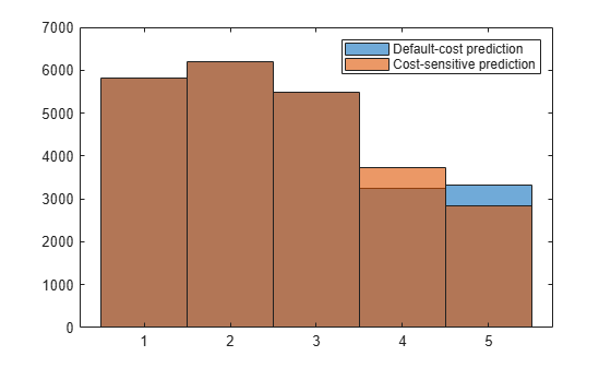
Because the cost-sensitive prediction method penalizes misclassifying class 4 so severely, more predictions into class 4 result as compared to the prediction method that uses the default, balanced cost.
Load the human activity data set. Randomly shuffle the data.
load humanactivity
n = numel(actid);
rng(10) % For reproducibility
idx = randsample(n,n);
X = feat(idx,:);
Y = actid(idx);
For details on the data set, enter Description at the command line.
Create a naive Bayes classification model for incremental learning. Specify the class names. Prepare the model for predict by fitting the model to the first 10 observations.
Mdl = incrementalClassificationNaiveBayes('ClassNames',unique(Y));
initobs = 10;
Mdl = fit(Mdl,X(1:initobs,:),Y(1:initobs));
canPredict = size(Mdl.DistributionParameters,1) == numel(Mdl.ClassNames)
canPredict = logical
1
Mdl is an incrementalClassificationNaiveBayes model. All its properties are read-only. The model is configured to generate predictions.
Simulate a data stream, and perform the following actions on each incoming chunk of 100 observations.
Call
predictto compute class posterior probabilities for each observation in the incoming chunk of data.Call
rocmetricsto compute the area under the ROC curve (AUC) using the class posterior probabilities, and store the AUC value, averaged over all classes. This AUC is an incremental measure of how well the model predicts the activities on average.Call
fitto fit the model to the incoming chunk. Overwrite the previous incremental model with a new one fitted to the incoming observations.
numObsPerChunk = 100;
nchunk = floor((n - initobs)/numObsPerChunk);
auc = zeros(nchunk,1);
classauc = 5;

% Incremental learning
for j = 1:nchunk
    ibegin = min(n,numObsPerChunk*(j-1) + 1 + initobs);
    iend   = min(n,numObsPerChunk*j + initobs);
    idx = ibegin:iend;
    [~,posterior] = predict(Mdl,X(idx,:));
    mdlROC = rocmetrics(Y(idx),posterior,Mdl.ClassNames);
    [~,~,~,auc(j)] = average(mdlROC,'micro');
    Mdl = fit(Mdl,X(idx,:),Y(idx));
end
Now, Mdl is an incrementalClassificationNaiveBayes model object trained on all the data in the stream.
Plot the AUC values for each incoming chunk of data.
plot(auc)
xlim([0 nchunk])
ylabel('AUC')
xlabel('Iteration')
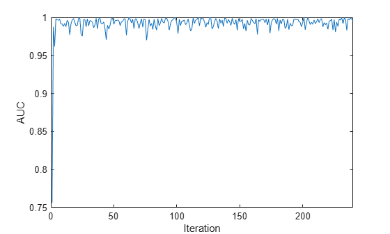
The plot suggests that the classifier predicts the activities well during incremental learning.
Input Arguments
Name-Value Arguments
Output Arguments
More About
Version History
Introduced in R2021a