fit
Train naive Bayes classification model for incremental learning
Description
The fit function fits a configured naive Bayes classification model for incremental learning (incrementalClassificationNaiveBayes object) to streaming data. To additionally track performance metrics using the data as it arrives, use updateMetricsAndFit instead.
To fit or cross-validate a naive Bayes classification model to an entire batch of data at once, see fitcnb.
Mdl = fit(Mdl,X,Y)Mdl, which represents the input naive Bayes classification model for
incremental learning Mdl trained using the predictor and response
data, X and Y respectively. Specifically,
fit updates the conditional posterior distribution of the
predictor variables given the data.
Examples
Fit an incremental naive Bayes learner when you know only the expected maximum number of classes in the data.
Create an incremental naive Bayes model. Specify that the maximum number of expected classes is 5.
Mdl = incrementalClassificationNaiveBayes('MaxNumClasses',5)Mdl =
incrementalClassificationNaiveBayes
IsWarm: 0
Metrics: [1×2 table]
ClassNames: [1×0 double]
ScoreTransform: 'none'
DistributionNames: 'normal'
DistributionParameters: {}
Properties, Methods
Mdl is an incrementalClassificationNaiveBayes model. All its properties are read-only. Mdl can process at most 5 unique classes. By default, the prior class distribution Mdl.Prior is empirical, which means the software updates the prior distribution as it encounters labels.
Mdl must be fit to data before you can use it to perform any other operations.
Load the human activity data set. Randomly shuffle the data.
load humanactivity
n = numel(actid);
rng(1) % For reproducibility
idx = randsample(n,n);
X = feat(idx,:);
Y = actid(idx);
For details on the data set, enter Description at the command line.
Fit the incremental model to the training data, in chunks of 50 observations at a time, by using the fit function. At each iteration:
Simulate a data stream by processing 50 observations.
Overwrite the previous incremental model with a new one fitted to the incoming observations.
Store the mean of the first predictor in the first class and the prior probability that the subject is moving (
Y> 2) to see how these parameters evolve during incremental learning.
% Preallocation
numObsPerChunk = 50;
nchunk = floor(n/numObsPerChunk);
mu11 = zeros(nchunk,1);
priormoved = zeros(nchunk,1);

% Incremental fitting
for j = 1:nchunk
    ibegin = min(n,numObsPerChunk*(j-1) + 1);
    iend   = min(n,numObsPerChunk*j);
    idx = ibegin:iend;
    Mdl = fit(Mdl,X(idx,:),Y(idx));
    mu11(j) = Mdl.DistributionParameters{1,1}(1);
    priormoved(j) = sum(Mdl.Prior(Mdl.ClassNames > 2));
end
Mdl is an incrementalClassificationNaiveBayes model object trained on all the data in the stream.
To see how the parameters evolve during incremental learning, plot them on separate tiles.
t = tiledlayout(2,1);
nexttile
plot(mu11)
ylabel('\mu_{11}')
xlabel('Iteration')
axis tight
nexttile
plot(priormoved)
ylabel('\pi(Subject Is Moving)')
xlabel(t,'Iteration')
axis tight
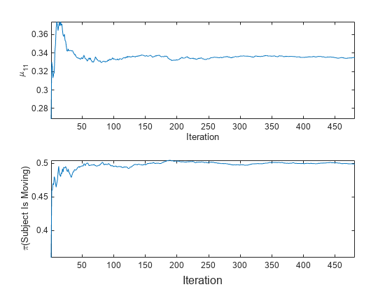
fit updates the posterior mean of the predictor distribution as it processes each chunk. Because the prior class distribution is empirical, (subject is moving) changes as fit processes each chunk.
Fit an incremental naive Bayes learner when you know all the class names in the data.
Consider training a device to predict whether a subject is sitting, standing, walking, running, or dancing based on biometric data measured on the subject. The class names map 1 through 5 to an activity. Also, suppose that the researchers plan to expose the device to each class uniformly.
Create an incremental naive Bayes model for multiclass learning. Specify the class names and the uniform prior class distribution.
classnames = 1:5;
Mdl = incrementalClassificationNaiveBayes('ClassNames',classnames,'Prior','uniform')
Mdl =
  incrementalClassificationNaiveBayes

                    IsWarm: 0
                   Metrics: [1×2 table]
                ClassNames: [1 2 3 4 5]
            ScoreTransform: 'none'
         DistributionNames: 'normal'
    DistributionParameters: {5×0 cell}


  Properties, Methods
Mdl is an incrementalClassificationNaiveBayes model object. All its properties are read-only. During training, observed labels must be in Mdl.ClassNames.
Mdl must be fit to data before you can use it to perform any other operations.
Load the human activity data set. Randomly shuffle the data.
load humanactivity
n = numel(actid);
rng(1); % For reproducibility
idx = randsample(n,n);
X = feat(idx,:);
Y = actid(idx);
For details on the data set, enter Description at the command line.
Fit the incremental model to the training data by using the fit function. Simulate a data stream by processing chunks of 50 observations at a time. At each iteration:
Process 50 observations.
Overwrite the previous incremental model with a new one fitted to the incoming observations.
Store the mean of the first predictor in the first class and the prior probability that the subject is moving (
Y> 2) to see how these parameters evolve during incremental learning.
% Preallocation
numObsPerChunk = 50;
nchunk = floor(n/numObsPerChunk);
mu11 = zeros(nchunk,1);
priormoved = zeros(nchunk,1);

% Incremental fitting
for j = 1:nchunk
    ibegin = min(n,numObsPerChunk*(j-1) + 1);
    iend   = min(n,numObsPerChunk*j);
    idx = ibegin:iend;
    Mdl = fit(Mdl,X(idx,:),Y(idx));
    mu11(j) = Mdl.DistributionParameters{1,1}(1);
    priormoved(j) = sum(Mdl.Prior(Mdl.ClassNames > 2));
end
Mdl is an incrementalClassificationNaiveBayes model object trained on all the data in the stream.
To see how the parameters evolve during incremental learning, plot them on separate tiles.
t = tiledlayout(2,1);
nexttile
plot(mu11)
ylabel('\mu_{11}')
xlabel('Iteration')
axis tight
nexttile
plot(priormoved)
ylabel('\pi(Subject Is Moving)')
xlabel(t,'Iteration')
axis tight
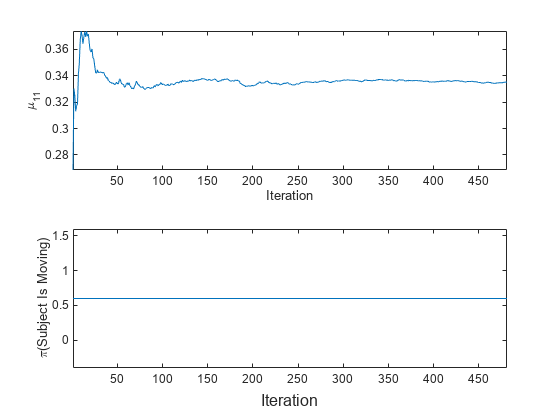
fit updates the posterior mean of the predictor distribution as it processes each chunk. Because the prior class distribution is specified as uniform, (subject is moving) = 0.6 and does not change as fit processes each chunk.
Train a naive Bayes classification model by using fitcnb, convert it to an incremental learner, track its performance on streaming data, and then fit the model to the data. Specify observation weights.
Load and Preprocess Data
Load the human activity data set. Randomly shuffle the data.
load humanactivity
rng(1); % For reproducibility
n = numel(actid);
idx = randsample(n,n);
X = feat(idx,:);
Y = actid(idx);
For details on the data set, enter Description at the command line.
Suppose that the data from a stationary subject (Y <= 2) has double the quality of the data from a moving subject. Create a weight variable that assigns a weight of 2 to observations from a stationary subject and 1 to a moving subject.
W = ones(n,1) + (Y <=2);
Train Naive Bayes Classification Model
Fit a naive Bayes classification model to a random sample of half the data.
idxtt = randsample([true false],n,true);
TTMdl = fitcnb(X(idxtt,:),Y(idxtt),'Weights',W(idxtt))
TTMdl =
ClassificationNaiveBayes
ResponseName: 'Y'
CategoricalPredictors: []
ClassNames: [1 2 3 4 5]
ScoreTransform: 'none'
NumObservations: 12053
DistributionNames: {1×60 cell}
DistributionParameters: {5×60 cell}
Properties, Methods
TTMdl is a ClassificationNaiveBayes model object representing a traditionally trained naive Bayes classification model.
Convert Trained Model
Convert the traditionally trained model to a naive Bayes classification model for incremental learning.
IncrementalMdl = incrementalLearner(TTMdl)
IncrementalMdl =
  incrementalClassificationNaiveBayes

                    IsWarm: 1
                   Metrics: [1×2 table]
                ClassNames: [1 2 3 4 5]
            ScoreTransform: 'none'
         DistributionNames: {1×60 cell}
    DistributionParameters: {5×60 cell}


  Properties, Methods
IncrementalMdl is an incrementalClassificationNaiveBayes model. Because class names are specified in IncrementalMdl.ClassNames, labels encountered during incremental learning must be in IncrementalMdl.ClassNames.
Separately Track Performance Metrics and Fit Model
Perform incremental learning on the rest of the data by using the updateMetrics and fit functions. At each iteration:
Simulate a data stream by processing 50 observations at a time.
Call
updateMetricsto update the cumulative and window minimal cost of the model given the incoming chunk of observations. Overwrite the previous incremental model to update the losses in theMetricsproperty. Note that the function does not fit the model to the chunk of data—the chunk is "new" data for the model. Specify the observation weights.Store the minimal cost.
Call
fitto fit the model to the incoming chunk of observations. Overwrite the previous incremental model to update the model parameters. Specify the observation weights.
% Preallocation
idxil = ~idxtt;
nil = sum(idxil);
numObsPerChunk = 50;
nchunk = floor(nil/numObsPerChunk);
mc = array2table(zeros(nchunk,2),'VariableNames',["Cumulative" "Window"]);
Xil = X(idxil,:);
Yil = Y(idxil);
Wil = W(idxil);

% Incremental fitting
for j = 1:nchunk
    ibegin = min(nil,numObsPerChunk*(j-1) + 1);
    iend   = min(nil,numObsPerChunk*j);
    idx = ibegin:iend;
    IncrementalMdl = updateMetrics(IncrementalMdl,Xil(idx,:),Yil(idx), ...
        'Weights',Wil(idx));
    mc{j,:} = IncrementalMdl.Metrics{"MinimalCost",:};
    IncrementalMdl = fit(IncrementalMdl,Xil(idx,:),Yil(idx),'Weights',Wil(idx));
end
IncrementalMdl is an incrementalClassificationNaiveBayes model object trained on all the data in the stream.
Alternatively, you can use updateMetricsAndFit to update performance metrics of the model given a new chunk of data, and then fit the model to the data.
Plot a trace plot of the performance metrics.
h = plot(mc.Variables);
xlim([0 nchunk])
ylabel('Minimal Cost')
legend(h,mc.Properties.VariableNames)
xlabel('Iteration')
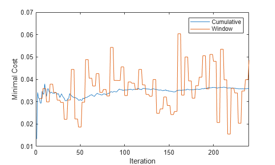
The cumulative loss gradually stabilizes, whereas the window loss jumps throughout the training.
Incrementally train a naive Bayes classification model only when its performance degrades.
Load the human activity data set. Randomly shuffle the data.
load humanactivity
n = numel(actid);
rng(1) % For reproducibility
idx = randsample(n,n);
X = feat(idx,:);
Y = actid(idx);
For details on the data set, enter Description at the command line.
Configure a naive Bayes classification model for incremental learning so that the maximum number of expected classes is 5, the tracked performance metric includes the misclassification error rate, and the metrics window size is 1000. Fit the configured model to the first 1000 observations.
Mdl = incrementalClassificationNaiveBayes('MaxNumClasses',5,'MetricsWindowSize',1000, ...
    'Metrics','classiferror');
initobs = 1000;
Mdl = fit(Mdl,X(1:initobs,:),Y(1:initobs));
Mdl is an incrementalClassificationNaiveBayes model object.
Perform incremental learning, with conditional fitting, by following this procedure for each iteration:
Simulate a data stream by processing a chunk of 100 observations at a time.
Update the model performance on the incoming chunk of data.
Fit the model to the chunk of data only when the misclassification error rate is greater than 0.05.
When tracking performance and fitting, overwrite the previous incremental model.
Store the misclassification error rate and the mean of the first predictor in the second class to see how they evolve during training.
Track when
fittrains the model.
% Preallocation
numObsPerChunk = 100;
nchunk = floor((n - initobs)/numObsPerChunk);
mu21 = zeros(nchunk,1);
ce = array2table(nan(nchunk,2),'VariableNames',["Cumulative" "Window"]);
trained = false(nchunk,1);

% Incremental fitting
for j = 1:nchunk
    ibegin = min(n,numObsPerChunk*(j-1) + 1 + initobs);
    iend = min(n,numObsPerChunk*j + initobs);
    idx = ibegin:iend;
    Mdl = updateMetrics(Mdl,X(idx,:),Y(idx));
    ce{j,:} = Mdl.Metrics{"ClassificationError",:};
    if ce{j,2} > 0.05
        Mdl = fit(Mdl,X(idx,:),Y(idx));
        trained(j) = true;
    end
    mu21(j) = Mdl.DistributionParameters{2,1}(1);
end
Mdl is an incrementalClassificationNaiveBayes model object trained on all the data in the stream.
To see how the model performance and evolve during training, plot them on separate tiles.
t = tiledlayout(2,1);
nexttile
plot(mu21)
hold on
plot(find(trained),mu21(trained),'r.')
xlim([0 nchunk])
ylabel('\mu_{21}')
legend('\mu_{21}','Training occurs','Location','best')
hold off
nexttile
plot(ce.Variables)
xlim([0 nchunk])
ylabel('Misclassification Error Rate')
legend(ce.Properties.VariableNames,'Location','best')
xlabel(t,'Iteration')
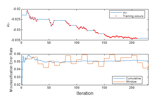
The trace plot of shows periods of constant values, during which the loss within the previous observation window is at most 0.05.
Input Arguments
Output Arguments
More About
Tips
Unlike traditional training, incremental learning might not have a separate test (holdout) set. Therefore, to treat each incoming chunk of data as a test set, pass the incremental model and each incoming chunk to
updateMetricsbefore training the model on the same data.