Dual-Motor Electric Vehicle Model using Powertrain Blockset™

A high-performance electric vehicle (EV) model with a dual-motor (2EM) architecture, developed using Powertrain Blockset™.

Dual-Motor Electric Vehicle Model using Powertrain Blockset™

This project features a high-performance electric vehicle (EV) model with a dual-motor (2EM) architecture, developed using Powertrain Blockset™. This model leverages a set of enhanced component models to achieve high-speed simulation, executing thousands of times faster than real-time.

This work requires MATLAB release R2024b or newer.

The model is parameterized using public specifications for Tesla Model 3 Long Range All-Wheel Drive (AWD) data and accurately defines traction forces and energy losses to estimate energy consumption and driving range. It includes a detailed comparison with published Tesla Model 3 Long Range AWD data, including energy consumption, driving range, and other key performance metrics.

Tesla Model 3 Long Range AWD Specifications

Parameter Value

Vehicle mass ~1830 kg (4030 lbs)

Aerodynamic drag coefficient (Cd) 0.23

Frontal area ~2.23 m²

Battery configuration 96s × 46p

Nominal battery voltage ~360 V

Battery capacity 75–82 kWh

Front motor peak torque 200 Nm @125-6375 rpm

Rear motor peak torque 350 Nm @325-5500 rpm

Max motor speed 18,000 rpm

Gear ratio (motor to wheels) ~9:1

Range ~557 km

Avg. energy consumption ~17.6 kWh/100 km

Energy efficiency ~6–7 km/kWh

0–100 km/h acceleration ~4.2 seconds

Top speed (limited) ~233 km/h

Although the Tesla Model 3 Long Range is used as the reference vehicle, the model is designed for easy reparameterization. By changing a few key inputs such as vehicle mass, motor specifications, battery size, and gear ratio, you can quickly simulate different EV configurations.

You can also configure different EV model architectures using the Virtual Vehicle Composer app. For more information, see Get Started with Virtual Vehicle Composer.

Use this model to support these engineering workflows:

• System-level design and optimization
• System sizing and component trade-off studies
• Longitudinal vehicle dynamics analysis
• Power consumption estimation and range studies
• Design space exploration of powertrain parameters

This demo shows you how to:

1. Parameterize an EV 2EM model using publicly available Tesla Model 3 Long Range AWD specifications.
2. Simulate transient drive cycles to validate the model’s accuracy against published energy consumption and range data.
3. Explore system sizing by varying key model parameters such as vehicle mass, motor specifications, and battery capacity.
4. Achieve high simulation speeds, enabling the model to be used in model-in-the-loop (MIL), hardware-in-the-loop (HIL), or automated optimization workflows.

Table of Contents

• Setup
• Simulation Model Overview
• Specify Model Parameters
• Run Simulation
• Plot Motor Efficiency
• Determine Simulation Speed
• Determine Maximum Velocity
• Power Consumption Analysis

Setup

To get started:

1. Download and unzip the files.
2. Open the project file LFM_EV_2EM.prj in MATLAB.
3. Then, open the Main.mlx live script located in the project’s root folder to begin exploring the model.

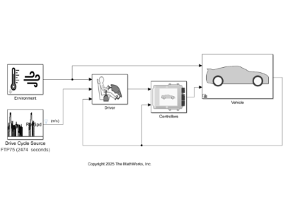
Simulation Model Overview

Open the LFM_EV_2EM project.

openProject("LFM_EV_2EM.prj");

The vehicle model includes these key components:

1. Vehicle Body Total Road Load with Load Transfer: Implements a one-degree-of-freedom (1DOF) rigid vehicle model using coast-down testing coefficients.

• Models the complete longitudinal road load dynamics, including aerodynamic drag, rolling resistance, road gradient, and dynamic load transfer between axles during acceleration and braking.

2. Simple Wheel: Simulates the longitudinal dynamics of the wheel-tire system. Optimized for fast execution with minimal parameterization. This block supports:

• Multiple rolling resistance modeling options
• Ability to disable wheel slip for faster simulations

3. Open Differential Driveline: Implements a kinematic open differential. This block allows:

• Power loss modeling via efficiency lookup tables or scalar values
• Specifying a damping coefficient as an alternative to efficiency modeling

4. Simple Gearbox Driveline: A simplified driveline model without gear inertias and downstream couplings. Supports drivetrain loss modeling via:

• Scalar damping coefficient
• Efficiency lookup table
• Scalar efficiency value

5. Datasheet Battery Model: Models battery behavior using:

• Open-circuit voltage (OCV) as a function of state of charge (SOC)
• Internal resistance as a function of SOC and temperature

6. Mapped Electric Motor: A system-level motor model that uses efficiency maps to represent:

• Motor torque-speed behavior
• Associated electrical efficiency/losses with torque, speed, temperature and voltage

7. Simple Thermal System: Regulates the temperatures of the battery, power electronics, motor, and cabin by generating heat flow rate demands and controlling them with PI control.

• Coefficient of Performance (COP) for the whole thermal management system is used for evaluating the efficiency efficiency of thermal management systems
• With only a minimal set of key parameters, it simplifies integration, calibration, and validation

Open the top level model.

modelName = "ConfiguredVirtualVehicleModel";
open_system(modelName);

Specify Model Parameters

All the default parameters are stored in the VirtualVehicleTemplate.sldd file. To parameterize this model, you can either edit values directly in the VirtualVehicleTemplate.sldd file using Model Exploer, or define custom data in the ParameterList.m. Open the ParamaeterList.m file. This file contains descriptions for each of the parameters it defines.

edit ParameterList.m

After specifying custom data in ParameterList.m, run these commands to open the top-level data dictionary, access the 'Design Data' section, import the custom data, and save the changes to the data dictionary.

if false %apply modified parameter values
    myDictionaryObj = Simulink.data.dictionary.open('VirtualVehicleTemplate.sldd');
    dDataSectObj = getSection(myDictionaryObj,'Design Data');
    importFromFile(dDataSectObj,'ParameterList.m','existingVarsAction','overwrite');
    saveChanges(myDictionaryObj);
end

Run Simulation

The model uses parameters based on the Tesla Model 3 Long Range, which has a catalog range of approximately 557 km and an EPA-rated energy efficiency of 6.5 to 6.7 km/kWh. These values vary depending on factors such as battery size, model variant, and driving conditions. Running the model through an FTP75 drive cycle yields an energy consumption of approximately 6.7 km/kWh and a driving range of 557 km, closely matching publicily available data for Tesla Model 3 Long Range. Run the simulation.

out = sim(modelName);

The results are displayed using the Simulation Data Inspector (SDI) tool.

Plot Motor Efficiency

Open and run the script, MotorEfficiencyPlot.mlx, to plot the front and rear motor efficiency for the drive cycle test.

edit MotorEfficiencyPlot;

Determine Simulation Speed

To evaluate simulation speed, select the checkbox to enable the functions to measure performance using the ratio of simulation time to elapsed wall time, exluding model initialization and termination phases.

if false
    simSpeed = (out.SimulationMetadata.ModelInfo.StopTime - out.SimulationMetadata.ModelInfo.StartTime)/...
        out.SimulationMetadata.TimingInfo.ExecutionElapsedWallTime    
end

As a simplified model, it runs approximately 1100 times faster than the wall clock time on a typical laptop. This efficiency makes it suitable for MIL simulation, HIL simulation (since it runs with a fixed-step solver), and system sizing optimization studies.

Determine Maximum Velocity

You can also verify the vehicle's maximum attainable velocity. The maximum speed of a Tesla Model 3 Long Range has a top speed that is electronically limited at approximately 233 km/h. The model reaches a top speed of 236 km/h. The 0 to 100 km/h (0 to 62 mph) acceleration time is approximately 4.2 seconds, which matches the published data of 4.2 seconds for the Tesla Model 3 Long Range. This validates the accuracy of the air resistance calculation model parameters, since this performance metric is mostly correlated with it.

Power Consumption Analysis

Open and run the script, GenerateEnergyReport.mlx, to generate the power consumption results.

edit GenerateEnergyReport;

MathWorks Products (http://www.mathworks.com)

Requires MATLAB® release R2024b.

• MATLAB® - required.
• Simulink™ - required.
• Stateflow® - required.
• Powertrain Blockset™ - required.

License

The license is available in the license.txt file within this repository.

Community Support

MATLAB Central

Project status

Last update: 10/15/2025

Copyright 2025 The MathWorks, Inc.