Techno-Economic Analysis of the Impact of EV Charging on the Power Grid
With techno-economic analysis, you can assess the technical feasibility and economic viability of electric vehicle charging infrastructure.
With more and more electric vehicles connecting to the power grid every day, there are concerns that existing grid infrastructure will be strained beyond acceptable operational limits. We can address these concerns by bringing operations, pricing, and forecasting into techno-economic models of power systems. Using these models, we can assess feasibility, risk, optimal operations, and profitability of charging infrastructure. These models provide key insights such as expected system performance over time, identification of factors that lead to bad outcomes, and right-sizing of components through optimization studies.
In this talk, we consider a scenario where a system operator can command individual electric vehicle battery units to both store and supply electricity while connected to the grid. The operator applies techno-economic optimization to the charging profiles to minimize electricity cost while accounting for system requirements and constraints, such as limits on state of charge, grid supply, and charge/discharge rate. The optimization provides a fast and automated approach for leveraging all of the units connected to the grid for overall system benefit. Charging profiles are then assessed for the impact on voltage and power flow levels using a grid-level simulation.
Published: 7 May 2023
Hello, and welcome to our talk on Techno-economic Analysis of the Impact of EV Charging on the Power Grid. Before we dive in, I'd like to introduce myself. My name is Ruth Anne Marchant. I'm a senior team lead based out of the Sydney, Australia office. I'm joined by my colleagues Graham Dudgeon and Chris Lee, and you'll have an opportunity to hear from them a little bit later.
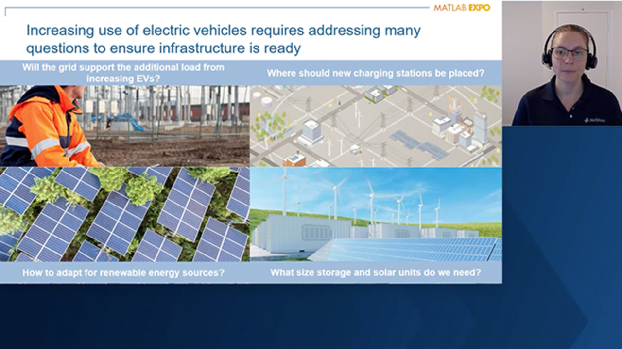
We'd like to encourage you to check out what others are saying on social media and share your excitement using the Matlab Expo hashtag. We'd also love to connect with you on LinkedIn. As more and more electric vehicles hit the road every day, there is concern about what impact this will have on our existing grid infrastructure. So the increasing use of electric vehicles requires us to investigate many questions to make sure that the infrastructure is ready.
These questions include, will the grid support the additional load from increasing EVs? Where should new charging stations be placed? How to adapt for renewable energy sources, and what size storage and solar units do we need? And there are many questions like this, but the underlying theme is that they're all targeted at reducing risk and building confidence in the resilience of grid infrastructure.
Addressing questions like this and the underlying concerns requires techno-economic analysis and optimization. Techno-economic analysis brings together both technical and economic considerations. Technical considerations can include looking at storage sizing, how equipment degrades over time, as well as contingency planning. And economic considerations could include things like energy prices, capital and operational expenditures, as well as business commitments that must be met.
By performing analysis and optimization that brings this all together, we can reduce risk, build confidence, and increase profitability. Techno-economic analysis helps us understand how our system will perform over time so we can identify problematic or risk factors and address them, as well as optimize the design and operation of the system. All of this can be done in an automated approach to address complex design and decision making scenarios.
MathWorks technology enables techno-economic analysis and optimization. We have many customers who have been very successful using our solutions for power systems analysis and design. Real world applications examples include developing virtual power plants, factory energy management systems, and other systems for optimizing power flow and energy production.
And we've seen that these studies at this scale are unique, with each organization having their own set of specific requirements and constraints. Off the shelf solutions may not fit the needs of the organization, so a solution built to address the specific requirements will often provide better results and insights. We provide the tools to build such solutions, including capabilities such as optimization, statistics, physical modeling, parallel computing, and more.
Together, these can be brought into techno-economic workflows, and we have multiple examples to illustrate this. Today we'll look at an example of using techno-economic optimization to study the impact of EV charging on grid infrastructure. We'll consider a scenario where we have multiple electric vehicles plugged into the system at different times. This type of scenario could present risk to the grid but also provides opportunities to explore innovative solution approaches.
We can explore possibilities like, what if charge scheduling accounted for electricity prices? What if EVs could also supply power to each other? And what if power could even be sold back to the grid? The plot in the middle here shows results from a scenario with just 20 vehicles. The red curve shows the grid power with just regular flat charging.
The yellow curve shows the grid power when we use optimization to apply a smart charging approach that limits the peak load and minimizes the total system cost. And the animation on the right illustrates more detailed analysis that we can do using a grid scale model to, for example, analyze the bus voltage across the entire network over time.
You can perform this type of techno-economic optimization in an end to end workflow, and we'll show that with this example. We'll start by modeling and solving an optimization problem based on energy balance. Then we'll perform more detailed analysis using grid simulation and visualization. And we'll finally discuss options to deploy this analysis workflow for others to use.
Thanks, Ruth Anne. So hi, everyone. My name is Chris Lee and I'm the senior product manager for our optimization products, and I'm based in Boston. So we want to explore how we can not only charge each EV storage unit, but leverage the units for overall system benefit while accounting for the price of electricity and even allowing power to be sold back to the grid. And we can model all of this as an optimization problem.
So we're assuming that we know the cost of power provided by the grid over time as well as the time intervals that each electric vehicle is plugged into the system over a 24 hour period. Now, the first step to setting up an optimization problem is defining the optimization variables, constraints, and objectives. And before I do that, I want to point out that in this example, we're not looking to prescribe the details of how you would solve this problem or even try to address the social aspects of implementing such a system.
And so we're not going to attempt to model every possible consideration here, but instead, the goal is to give you an idea of what's possible with the tools we provide. So our optimization variables include the power going in and out of each of the EV storage units, as well as the power bought from and sold to the grid. There are multiple technical constraints that we'll consider.
The state of charge for each unit must stay between certain limits, and the final state of charge of each unit must be fully charged by the time the vehicle is unplugged. We're modeling our system using energy balance, and so the grid power must be balanced with the storage unit power and the system load power. And finally, the grid power itself also has certain upper and lower limits.
Those were the technical aspects of the problem. The economic portion of this problem is in the objective function, where we are minimizing the total cost of electricity for the full system. Next we need to translate our problem into an optimization model in Matlab code. Matlab provides an approach called the problem based optimization workflow, which is a really intuitive process to go from the problem that we just described to the Matlab implementation, and I'll illustrate this with a few examples.
So one of our variables was the power bought from or sold to the grid. Mathematically, this means that grid power is a continuous quantity with some minimum and maximum bounds. And so in Matlab we define grid power as a so-called optimization variable and provide its name, its size, which in this case is the number of time steps, and values for the lower and upper bounds.
One of the constraints is that the grid power must be balanced with the storage unit and system load power, and this means that the sum of all the storage powers plus the load power must equal the grid power. And the Matlab code that defines this constraint expression looks just like that, and it also includes the grid power variable that we created earlier.
Our objective is to minimize the total cost of electricity. The total cost is obtained by multiplying the grid power times the price of power over the whole time, and you can see how in Matlab we define the objective expression in the same way. And for the rest of the problem, we would implement the other variables and constraints with the same approach and then solve the problem by calling the solve function.
And the solve function automatically determines the appropriate optimization solver to use based on the problem that you've defined. In this case, we're solving a linear program. So this problem based optimization workflow makes it really easy for users to both implement and understand the optimization model, and it also makes it easy to gradually build up the problem. For example, incrementally adding new constraints along the way.
So let's take a look at some results. Each unit is plugged in at different times and for different durations, and you can see that with smart charging determined by the optimization, the state of charge does not ramp up uniformly as it does with a constant charge approach. In some cases, the state of charge actually decreases as the vehicle unit is supplying power, either to other vehicles or even back to the grid. And this helps achieve overall system benefit.
The charge profiles still satisfy the lower and upper bound constraints, as well as the requirement that each unit be fully charged at the end of its plugin duration. Here the blue curve shows the total grid power over the full time period using smart charging. You can see that the power does not exceed 50 kilowatts in this case, and toward the end the power actually drops and goes negative, indicating that power is being fed back into the grid.
So at this point, the optimization has determined that selling some power back to the grid at this time period is beneficial because the price of electricity is at its highest, as you can see with the red curve. And in this case, the overall result is a 6.2% cost savings for the entire system. Here, again, we compare the flat charging profile with the optimized charging profile.
And so by using optimization, we've achieved a technical benefit of reduced peak load as well as an economic benefit of cost savings for this for the full system. Now up to this point, we've only been showing results for a scaled down version of the study with just 20 electric vehicles in the system just to make things easier to see, but we can scale this up.
So the full scale study includes 906 units, which is representative of the IEEE European test feeder. And even at this scale, the optimization took just 20 seconds to solve on my laptop. The optimization, again, reduces the peak load and provides cost savings for the system by selling power back to the grid when the price is high. So next I'll pass things off to Graham to talk about the next step of the workflow, which is grid simulation.
Hello, everyone. My name is Graham Dudgeon, and I am principal product manager for electrical technology at MathWorks. In this section, we'll consider how we enhance our engineering study by evaluating the charging responses on a full power grid simulation. We choose the IEEE European test feeder, as it's a relatively large grid scale model with published benchmark results. The IEEE European test feeder is a 906 plus 3 phase radial feeder, which, as published, has 55 unbalanced loads.
The system is published by the IEEE AMPS distribution system analysis subcommittee. You may download the network data at the link shown. As there are 906 three phase buses, we have 2,718 nodes. We'll adjust this model so that a storage device may be placed on any node. If you want to download scripts to build the IEEE European test feeder automatically using Simscape Electrical and then run the model against the published benchmark response, then please visit MathWorks File Exchange.
For the greatest flexibility with scenario evaluation, we place a bidirectional power input at each node where we can input a given power profile as time series data. For this system, we have 2,718 possible power inputs. What I'm showing on the right is how we implement active and reactive power inputs on each node at a given bus. Note that the scenarios that we're considering in this presentation, we will use only active power inputs.
Our first scenario is where each of the 2,718 nodes has a storage unit, each with random plugin duration, and we optimize each phase separately. There are 906 storage units per phase. As we are simulating over a 24 hour period and are interested in the system response at 10 minute intervals, we implement the simulation as a phasor or RMS simulation.
We choose a time step of five minutes, as our power inputs require an algebraic loop brake, which is implemented in this case as a unit delay. This is a so-called quasi steady simulation, where there are no dynamics modeled in the electrical system and we can rapidly move from one operating point to the next. What we're looking at here is a substation active power on a pair phase basis. You can see the similarity between these profiles and what was shown earlier.
Note the differences that you see in each phase are primarily due to different plugin durations. With a grid simulation, we also have access to voltage and current profiles. Here we're looking at voltage and phase A across 10 nodes. Note with the smart profile how voltage drops when there is overall power consumption and how voltage then increases when there is overall power supply. As the flat profile is only consumption, the voltages drop accordingly.
In this section, we'll consider how we efficiently simulate multiple scenarios and how we may visualize large amounts of data. In this scenario, we'll assess aggregated storage units connected to a single bus, and we wish to assess each bus separately. We therefore have 906 scenarios to evaluate. Specifically, we want to look at the power demand that the substation for each location. Using parallel computing, we can evaluate multiple scenarios in a time efficient manner.
The figure on the left shows a histogram of the maximum active power demand at the substation for each location. I'll talk more about this in a moment. On the right, you're seeing a sped up view of running the 906 scenarios on multiple course. The 906 scenarios took approximately 30 minutes to run, which is about two seconds per scenario. This is a 3.5 time speed up when using four cores. The more cores you have, the greater the speedup will be.
The histogram on the left shows the distribution of substation maximum power as a function of charging location. The graph on the right shows the network. You can see that the substation is located at the top left. I've also color coded the charging locations as a function of the maximum power demand at the substation. The further we locate ourselves from the substation, the more power needs to be delivered due to increased losses in the cables. This is expected.
As can be seen in this example, locating the charging station at the most distant bus results in 1.9% more power being required from the substation. This, of course, assumes that we are not considering local generation sources at the charging station. That's a topic for another time.
This animation shows the voltage level of each bus across a 24 hour period for one charging scenario. Notice the voltage fluctuations when the substation power is constant. This is due to the local variance in the charging patterns. Also note that when the substation power goes negative, indicating supply back to the grid, that the voltage levels increase.
In this section, we'll discuss deployment options for applications, algorithms, and simulation models. MathWorks offers a range of options to deploy your applications, algorithms, and simulation models depending on your specific needs. You can deploy algorithms to embedded hardware such as microprocessors, FPGAs, PLCs, and GPUs using our code or products.
You can deploy applications to the desktop and the web using Matlab Compiler, and to enterprise systems through Matlab Compiler SDK. Simulink Compiler provides a deployment path for simulation models, including some scale models. Applications for simulation models can include web deployment of digital twins.
Here are our key takeaways. You can reduce risk and build confidence in power grid readiness through techno-economic analysis. You can model and solve large scale optimization studies using problem based modeling. You can craft your problem to use efficient solvers such as linear programming. You can expand engineering studies by performing grid simulations and enhance your understanding of the system response with statistical analysis and visualization. And you can operationalize your analysis and simulation workflows through a broad range of deployment options.
MathWorks offers a range of resources to support you in the use of our software for specific application areas. You can check out examples in our documentation or visit MathWorks File Exchange to see examples from both MathWorks staff and our user community. You can access free self-paced training or attend instructor led training. Finally, our consulting team can support you with the adoption of our software and help meet your specific project needs. We hope you found this session valuable. Thank you for listening.
Related Products
Learn More
Featured Product
Global Optimization Toolbox
Up Next:

Related Videos:


Select a Web Site
Choose a web site to get translated content where available and see local events and offers. Based on your location, we recommend that you select: United States.
You can also select a web site from the following list
Americas
- América Latina (Español)
- Canada (English)
- United States (English)
Europe
- Belgium (English)
- Denmark (English)
- Deutschland (Deutsch)
- España (Español)
- Finland (English)
- France (Français)
- Ireland (English)
- Italia (Italiano)
- Luxembourg (English)
- Netherlands (English)
- Norway (English)
- Österreich (Deutsch)
- Portugal (English)
- Sweden (English)
- Switzerland
- United Kingdom (English)